3 Basic R
3.1 Vectors, fuctions and variables
3.1.1 Doing Math in the console
The console is the place where you do quick calculations, tests and analyses that do not need to be saved (yet) or repeated. It is the the tab that says “Console” and on first use, R puts it in the lower left panel.
In the console, the prompt is the “greater than” symbol “>”. R waits here for you to enter commands. When the panel has “focus” the cursor is blinking on and off. You can use the console as a calculator. It supports all regular math operations, in the way you would expect them:
+ : ‘plus’, as in 2 + 2 = 4
- : ‘subtract’, as in 2 - 2 = 0
* : ‘multiply’, as in 2 * 3 = 6
/ : ‘divide’, as in 8 / 4 = 2
^ : ‘exponent’, as in 2^3 = 8. In R, ^ is synonym of **
For the square root you can use \(n^{0.5}\): n**0.5, or the function sqrt() (discussed later).
When Enter is pressed when the mathematical statement is not complete yet, the > symbol is replaced by a + at the start of the new line, indicating the statement is a continuation. Here is an example:
> 1 + 3 + 4 +
+
So the + at the start of line 2 is not a mathematical + but a “continuation symbol”. You can always abort the current statement by pressing Escape.
When a statement is complete, the result will be printed in the next line:
> 31 + 11
[1] 42
The result is of course 42; the leading [1] is the index of the result. We will address this later.
Operator Precedence
All “operators” adhere to the standard mathematical precedence rules (PEMDAS):
    Parentheses (simplify inside these)
    Exponents
    Multiplication and Division (from left to right)
    Addition and Subtraction (from left to right)
With complex statements you should be aware of operator precedence! If you are not sure, or want to make your expression less ambiguous you should simply use parentheses () because they have highest precedence.
Besides math operators, R knows a whole set of other operators. They will be dealt with later in this chapter.
Programming Rule Always place spaces around both sides of an operator, with the exception of
^and**.
3.1.2 An expression dissected
When you type 21 / 3 this called an expression. The expression has three parts: an operator (/ in the middle) and two operands. The left operand is 21 and the right operand is 3.
Since there is no assignment, the result of this expression will be send to the console as output, giving [1] 7.
Because this expression is the sole contents of the current line in the console, it is also called a statement.
Statement vs expression A statement is a complete line of code that performs some action, while an expression is any section of code that evaluates to a value.
Ending statements
In R, the newline (enter) is an end-of-statement character. Optionally you can end statements with a semicolon “;”. However, when you have more statements on a single line they are mandatory is in this example:
x <- c(1, 2, 3); x; x <- 42; x## [1] 1 2 3## [1] 42Programming Rule: Have one statement per line and don’t use semicolons
3.1.3 Functions
Simple mathematics is not the core business of R.
Going further than basic math, you will need functions, mostly pre-existing functions but often also custom functions that you write yourself. Here is a definition of a function:
A function is a piece of functionality that you can execute by typing its name, followed by a pair of parentheses. Within these parentheses, you can pass data for the function to work on. Functions often, but not always, return a value.
Function usage -or a function call- has this general form: \[function\_name(arg_1, arg_2, ..., arg_n)\]
Example: Square root with sqrt()
You have already seen that the square root can be calculated as \(n^{0.5}\).
However, there is also a function for it: sqrt(). It returns the square root of the given parameter, a number, e.g. sqrt(36)
36^0.5
sqrt(36)
## [1] 6
## [1] 6Another example: paste()
The paste() function can take any number of arguments and returns them, combined into a single text (character) string. You can also specify a separator using sep="<separator string>":
paste(1, 2, 3, sep = "---")## [1] "1---2---3"Note the use of quotes surrounding the dashes: "---"; they indicate it is text, or character, data.
Also note the use of a name for only the last argument. Not all arguments can be specified by name, but when possible this has preference, as in sep = "---".
3.1.3.1 Getting help on a function
Type ?function_name or help(function_name) in the console to get help on a function. The function documentation will appear in the panel containing the Help tab, Its location is dependent on your set of preferences.
For instance, typing ?sqrt will give the help page of the square root function together with the abs() function.
R help pages always have the exact same structure:
- Name & package (e.g.
{base}) - Short description
- Description
- Usage
- Arguments
- Details
- …
- Examples
Scroll down in the help to see example usages of the function. Alternatively, type example(sqrt) in the console to have all examples executed in order, until you press Escape.
3.1.4 Variables
In math and programming you often use variables to label or name pieces of data, or a function in order to have them reusable, retrievable, changeable.
A variable is a named piece of data stored in memory that can be accessed via its name
For instance, x = 42 is used to define a variable called x, with a value attached to it of 42. Variables are really variable - their value can change!
In R you usually assign a value to a variable using “<-”, so “x <- 42” is equivalent to “x = 42”. Both will work in R, but the “arrow” notation is preferred.
3.1.5 Vectors
R is completely vector-based
In R, all data lives inside vectors. When you type ‘2 + 4’, R will execute the following series of actions:
- create a vector of length 1 with its element having the value 2
- create a vector of length 1 with its element having the value 4
- add the value of the second vector to ALL the values of vector one, and recycle any shorter vector as many times as needed
Step 3 is a crucial one. It is essential to grasp this aspect in order to understand R. Therefore we’ll revisit it later in more detail.
The atomic datatypes
R knows five basic types of data; other datatypes are build by combining these into more complex structures (discussed in a later chapter):
| type | descripton | examples |
|---|---|---|
| numeric | numbers with a decimal part |
3.123, 5000.0, 4.1E3
|
| integer | numbers without a decimal part |
1, 0, 2999
|
| logical | Boolean values: yes/no) |
true false
|
| character | text, should be put within quotes |
'hello R' "A cat!"
|
| factor | nominal and ordinal scales | <dealt with later> |
All these types are created in similar ways and can often be converted into other types.
Note 1: If you type a number in the console, it will always be a numeric value, decimal part or not.
Note 2: For character data, single and double quotes are equivalent but double are preferred; type ?Quotes in the console to read more on this topic.
Note 3: There are also date/time types but they are not discussed here
Creating vectors
You will see shortly that there are many ways to create vectors: a custom collection, a series, a repetition of a smaller set, a random sample from a distribution, etc. etc.
The simplest way to create a vector is the first: create a vector from a custom set of elements, using the “Concatenate” function c(). The c() function simply takes all its arguments and puts them behind each other, in the order in which they were passed to it, and returns the resulting vector.
## [1] 2 4 3## [1] "a" "b" "c" "d"## [1] 0.100 0.010 0.001## [1] TRUE FALSE TRUE FALSEVectors can hold only one data type
A vector can hold only one type of data. Therefore, if you pass a mixed set of values to the function c(), it will coerce all data into one type. The preferred type is numeric. However, when that is not possible the result will most often be a character vector. In the example below, two numbers and a character value are passed. Since "a" cannot be coerced into a numeric, the returned vector will be a character vector.
c(2, 4, "a") ## [1] "2" "4" "a"Here are some more coercion examples.
## [1] 1 2 1## [1] "TRUE" "FALSE" "TRUE"## [1] "1.3" "TRUE" "1"Using the function class(), you can get the data type of any value or variable.
## [1] "character"## [1] "integer"## [1] "numeric"## [1] "numeric"Vector arithmetic
Let’s have a look at what it means to work with vectors, as opposed to singular values (also called scalars). An example is probably best to get an idea.
## [1] 8 6 9 7As you can see, R works set based and will cycle the shorter of the two operands to deal with all elements of the longer operand. How about when the longer one is not a multiple of the shorter one?
## Warning in x - z: longer object length is not a multiple of shorter object
## length
## [1] 1 2 0 4As you can see this generates a warning that “longer object length is not a multiple of shorter object length”. However, R will proceed anyway, cycling the shorter one.
3.1.6 Operators
Here is a complete listing of operators in R. Some operators such as ^ are unary, which means they have a single operand; a single value or they operate on. On the other hand, binary operators such as + have two operands.
The following unary and binary operators are listed in precedence groups, from highest to lowest. Many of them are still unknown to you of course. We will encounter most of these along the way as the course progresses, starting with a few in this section.
| operator | purpose |
|---|---|
| :: ::: | access variables in a namespace |
| $ @ | component / slot extraction |
| [ [[ | indexing |
| ^ | exponentiation (right to left) |
| - + | unary minus and plus |
| : | sequence operator |
| %any% | special operators (including %% and %/%) |
| * / | multiply, divide |
| + - | (binary) add, subtract |
| < > <= >= == != | ordering and comparison |
| ! | negation |
| & && | and |
| | || | or |
| ~ | as in formulae |
| -> ->> | assignment (left to right) |
| <- <<- | assignment (right to left) |
| = | assignment (right to left) |
| ? | help (unary and binary) |
The <<- assignment operator is the same as <- but assigns to a variable in the Global environment.
Logical operators
Logical operators are used to evaluate and/or combine expressions that result in a single logical value: TRUE or FALSE. The comparison operators compare two values (numeric, character - any type is possible) to get to a logical value, but always set-based! In the following chunk, each of the values in x is considered and if it is smaller than or equal to the value 4, TRUE is returned, else FALSE.
x <- c(1, 5, 4, 3)
x <= 4
## [1] TRUE FALSE TRUE TRUEOther comparison operators are < (less then), <= (less then or equal to), > (greater then), >= (greater then or equal to), and == (equal to).
Another category of logical operators is the set of boolean operators. These are used to reduce two logical values into one. These are
-
&: logical “AND”;a & bwill evaluate toTRUEonly ifaANDbare TRUE.
-
|: logical “OR”;a | bwill evaluate toTRUEonly ifaORbare TRUE, no matter which. -
!: logical -unary- “NOT”; negates the right operand:! awill evaluate to the “flipped” logical value ofa.
Here is a more elaborate example combining comparison and boolean operators.
Suppose you have vectors a and b and you want to know which values in a are greater than in b and also smaller than 3. This is the expression used for answering that question.
a <- c(2, 1, 3, 1, 5, 1)
b <- c(1, 2, 4, 2, 3, 0)
a > b & a < 3 ## returns a logical vector with test results
## [1] TRUE FALSE FALSE FALSE FALSE TRUEHere is a special case. Can you figure out what happens there?
6 - 2 : 5 < 3## [1] FALSE FALSE TRUE TRUECalculations with logical vectors
Quite often you want to know how many cases fit some condition. A convenient thing in that case is that logical values have a numeric counterpart or “hidden face”:
- TRUE == 1
- FALSE == 0
The sum() function is often used on this feature:
x <- c(2, 4, 2, 1, 5, 3, 6)
x > 3 ## which values are greater than 3?
sum(x > 3) ## how many are greater than 3?
## [1] FALSE TRUE FALSE FALSE TRUE FALSE TRUE
## [1] 3Modulo: %%
The modulo operator gives the remainder of a division.
## [1] 1
## [1] 0
## [1] 2
The modulo is most often used to establish periodicity: x %% 2 is zero for all even numbers. Likewise, x %% 10 will be zero for every tenth value.
Integer division %/% and rounding
The integer division is the complement of modulo and gives the integer part of a division, it simply “chops off” the decimal part.
## [1] 3
## [1] 2
## [1] 3
Note that floor() does the same. In the same manner, ceiling() rounds up to the nearest integer, no matter how large the decimal part. Finally, there is the round() method to be used for - well, rounding. Be aware that rounding in R is not the same as rounding your course grade which always goes up at x.5. Rounding x.5 values mathematically goes to the nearest even number:
## [1] 0 2 2 4 4 6 6 8The %in% operator
The %in% operator is very handy when you want to know if the elements of one vector are present in another vector. An example explains best, as usual:
## [1] FALSE  TRUE  TRUE
## [1] FALSE  TRUE FALSE  TRUE
There is no positional evaluation, it simply reports if the corresponding element in the first is present anywhere in the second.
Selecting vector elements
You often want to get to know things about specific values within a vector
- what value is at the third position?
- what is the highest value?
- which positions have negative values?
- what are the last 5 values?
There are two principal ways to do this: through indexing with positionional reference (“addresses”) and through logical indexing.
Here is a picture that demonstrates both.
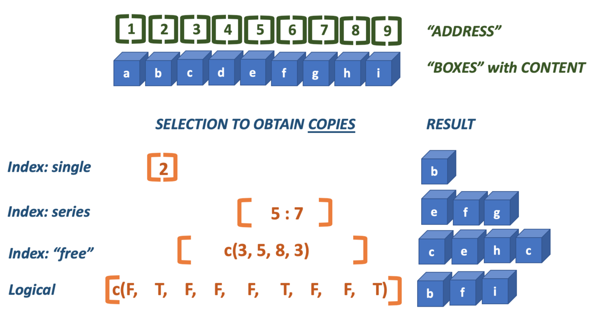
The index is the position of a value within a vector. R starts at one (1), and therefore ends at the length of the vector. Brackets [] are used to specify one or more indices that should be selected (returned).
Here are two examples of straightforward indexing, selecing a single or a series of elements.
x <- c(2, 4, 6, 3, 5, 1)
x[4] ## fourth element
## [1] 3
x[3:5] ## elements 3 to 5## [1] 6 3 5However, the technique is much more versatile. You can use indexing to select elements multiple times and thus create copies of them, or select elements in any order you desire.
x[c(1, 2, 2, 5)] ## elements 1, 2, 2 and 5## [1] 2 4 4 5
x <- c(2, 4, 6, 3, 5, 1)Besides integers you can use logicals to perform selections:
x[c(T, F, T, T, T, F)]## [1] 2 6 3 5As with all vector operations, shorter vectors are cycled as often as needed to cover the longer one:
x[c(F, T, F)]## [1] 4 5In practice you won’t type literal logicals very often; they are ususaly the result of some comparison operation. Here, all even numbers are selected because their modulo will retun zero.
x[x %% 2 == 0]## [1] 2 4 6And all of the maximum values in a vector are retreived:
## [1] 3 3 3There is a caveat in selecting the last n values: the colon operator has highest precedence! Here, the last two elements are (supposed to be selected).
## [1] 5 3 6 4 2## [1] 5 13.1.7 Vector creation methods
Since vectors are the bricks with which everything is built in R, there are many, many ways to create them. Here, I will review the most important ones.
Method 1: Constructor functions
Often you want to be specific about what you create: use the class-specific constructor OR one of the conversion methods. Constructor methods have the name of the type. They will create and return a vector of that type wit as length the number that is passed as constructor argument:
## [1] 0 0 0 0
## [1] "" "" "" ""
## [1] FALSE FALSE FALSE FALSE
Method 2: Conversion functions
Conversion methods have the name as.XXX() where XXX is the desired type. They will attempt to coerce the given input vector into the requested type.
x <- c(1, 0, 2, 2.3)
class(x)
as.logical(x)
as.integer(x)
## [1] "numeric"
## [1] TRUE FALSE TRUE TRUE
## [1] 1 0 2 2But there are limits to coercion: R will not coerce elements with types that are non-coercable: you get an NA value.
x <- c(2, 3, "a")
y <- as.integer(x)
## Warning: NAs introduced by coercion
class(y)## [1] "integer"
y## [1] 2 3 NAMethod 3: The colon operator
The colon operator (:) generates a series of integers fromthe left operand to -and including- the right operand.
1 : 5
5 : 1
2 : 3.66
## [1] 1 2 3 4 5
## [1] 5 4 3 2 1
## [1] 2 3Method 4: The rep() function
The rep() function takes three arguments. The first is an input vector. The second, times =, specifies how often the entire input vector should be repeated. The second argument, each =, specifies how often each individual element from the input vector should be repeated. When both arguments are provided, each = is evaluated first, followed by times =.
rep(1 : 3, times = 3)## [1] 1 2 3 1 2 3 1 2 3
rep(1 : 3, each= 3)## [1] 1 1 1 2 2 2 3 3 3
rep(1 : 3, times = 2, each = 3)## [1] 1 1 1 2 2 2 3 3 3 1 1 1 2 2 2 3 3 3Method 5: The seq() function
The seq() function is used to create a numeric vector in which the subsequent element show sequential increment or decrement. You specify a range and a step which may be neative if the range end (to =) is lower than the range start (from =).
## [1] 1.0 1.2 1.4 1.6 1.8 2.0 2.2 2.4 2.6 2.8 3.0## [1] 1.0 1.2 1.4 1.6 1.8 2.0## [1] 1.00 0.75 0.50 0.25 0.00## [1] 3 2 1 0Method 6: Through vector operations
Of course, new vectors, often of different type, are created when two vectors are combined in some operation, or a single vector is processed in some way.
This operation of two numeric vectors results in a logical vector:
1:5 < c(2, 3, 2, 1, 4)## [1] TRUE TRUE FALSE FALSE FALSEAnd this paste() call results in a character vector:
paste(0:4, 5:9, sep = "-")## [1] "0-5" "1-6" "2-7" "3-8" "4-9"3.1.8 Matrices are vectors with dimensions
We will not detail on them in this course, only this one small paragraph. This does not mean they are not important, but they are just not the focus here. Some functions require or return a matrix so you should be aware of them.
m <- matrix(1:10, nrow = 2, ncol = 5)
m
## [,1] [,2] [,3] [,4] [,5]
## [1,] 1 3 5 7 9
## [2,] 2 4 6 8 10## [,1] [,2] [,3] [,4] [,5]
## [1,] 1 3 5 7 9
## [2,] 2 4 6 8 10You can convert to and from dataframes using as.data.frame() and as.matrix(). From and to simple vectors is removing or adding dimension attributes: dim(m) <- NULL.
3.2 R embedded plot types (optional)
This section is included for completeness’ sake. The base plotting system can be considered deprecated.
You should preferably use the ggplot2 package for plotting.
Looking at numbers is boring - people want to see pictures! Doing analyses without visualizations is like only listening to a movie.
There are a few plot types supported by base R that deal with (combinations of) vectors:
- scatter (or line-) plot
- barplot
- histogram
- boxplot
We’ll only look at the bare basics in this chapter because we are going to do it for real with package ggplot2 in the next course.
3.2.1 Scatter and line plots
Meet plot() - the workhorse of R plotting.
time <- c(1, 2, 3, 4, 5, 6)
response <- c(0.09, 0.30, 0.41, 0.48, 0.72, 1.12)
plot(x = time, y = response)
Figure 3.1: Here is a nice figure!
The function plot is used here to generate a scatter plot. It may generae other types of figures, depending on its input as we’ll see later.
Formula notation
Instead of passing an x = and y = set of arguments, it is also possible to call the plot fuction with a formula notation:
plot(response ~ time)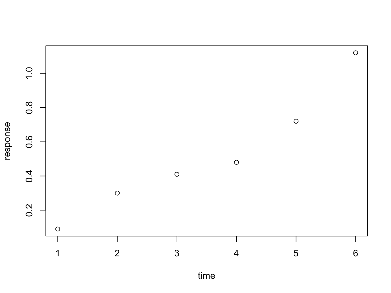
You can read response ~ time as response as a function of time. This is a nice, readable alternative in this case, but for many functions it is the only or preferred way to specify the relationship you want to investigate.
Plot decorations
Plots should always have these decorations:
- Axis labels indicating measurement type (quantity) and its units. E.g. ‘[Mg] (mq/ml)’ or ‘Heartrate (bpm)’.
- If multiple data series are plotted: a legend
- Either a title or a figure caption, depending on the context.
The first plots of this chapters were very bare (and a bit boring to look at): the plot has no axis labels (quantity and units) and no decoration whatsoever. By passing arguments to plot() you can modify or add many features of your plot. Basic decoration includes
- adjusting markers (
pch = 19,col = "blue") - adding connector lines (
type = "b") or removing points (type = "l") - adding axis labels and title (
xlab = "Time (hours)",ylab = "Systemic response",main = "Systemic response to agent X") - adjusting axis limits (
xlim = c(0, 8))
This is not an exhaustive listing; these are listed in the last section of this chapter.
Here is a more complete plot using a variety of arguments.
plot(x = time, y = response, pch = 19, type = "b", xlim = c(0, 8),
     xlab = "Time (hours)", ylab = "Systemic response (a.u.)",
     main = "Systemic response to agent X", col = "blue")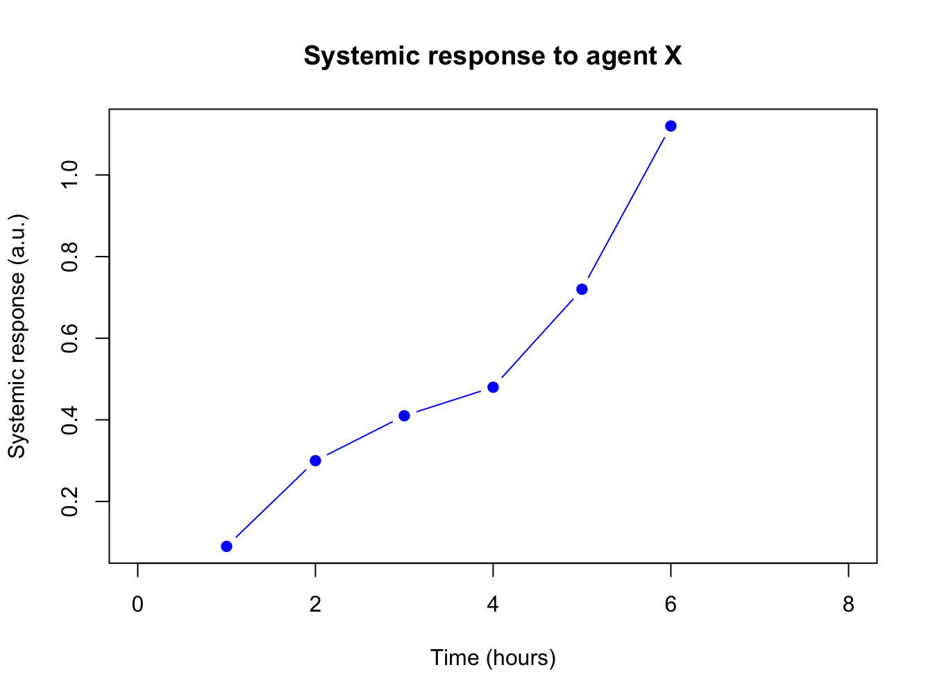
Adjusting the plot symbol
When you have many data points they will overlap. Using transparency with the rgb(,, alpha=) color definition and/or smaller plot symbols (cex=) solves this.
x <- rnorm(1000, 10, 2); y <- x + rnorm(1000, 0.5, 0.5)
plot(x, y, pch = 19, cex = 0.6,
     col = rgb(red = 0, green = 0, blue = 1, alpha = 0.2))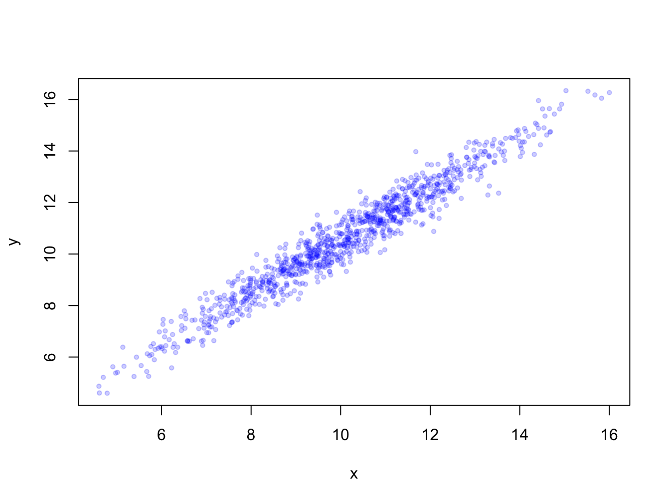
3.2.2 Barplots
Barplots can be generated in several ways:
- By passing a factor to
plot()- it will generate a barplot of level frequencies. This is a shorthand forbarplot(table(some_factor)). - By using
barplot(). The advantage of this is that accepts some graphical parameters that are not relevant and accepted byplot(), such asbeside =,height =,width =and others (type?barplotto see all).
Here is an example:
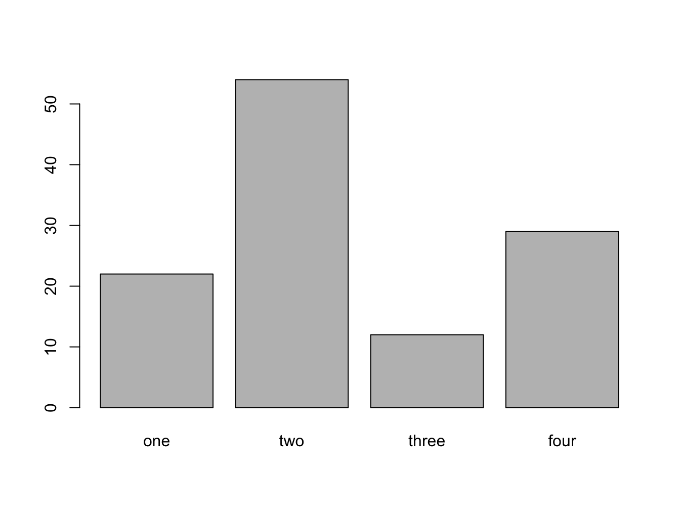
barplot() with a vector
The function barplot() can be called with a vector specifying the bar heights (frequencies), or a table object.
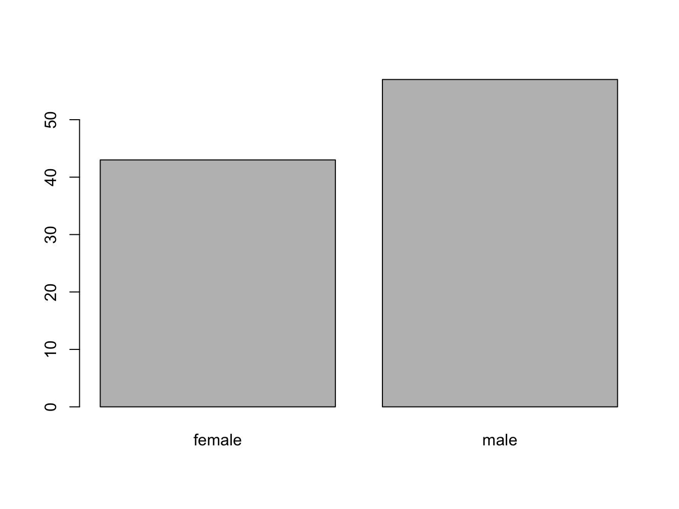
With a table object:
table(persons)## persons
## female male
## 43 57
barplot() with a 2D table object
Suppose you have this data:
set.seed(1234)
course <- rep(c("biology", "chemistry"), each = 10)
passed <- sample(c("Passed", "Failed"), size = 20, replace = T)
tbl <- table(passed, course) # the order matters!
tbl
## course
## passed biology chemistry
## Failed 6 8
## Passed 4 2The set.seed(1234) makes the sampling reproducible, although that sounds really unlogical. Discussing pseudorandom sampling is not within the scope of this course however.
You can create a stacked bar chart like this.
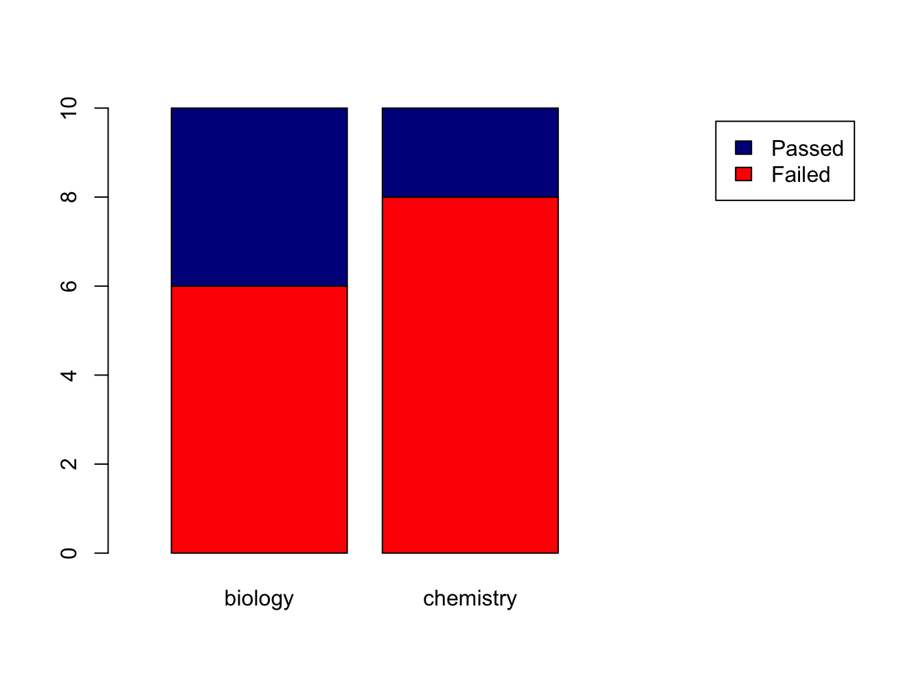
The xlim = setting is a trick to get the legend beside the plot.
Using the beside = TRUE argument, you get the bars side by side:
barplot(tbl,
        col=c("red", "darkblue"),
        beside = TRUE,
        xlim=c(0, ncol(tbl)*2 + 3),
        legend = rownames(tbl))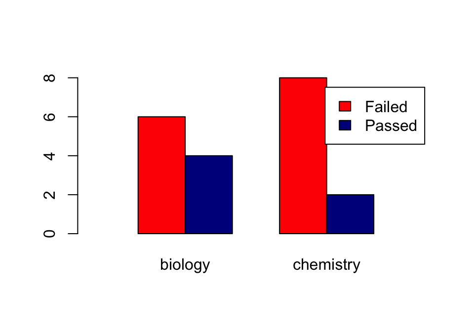
Later, we’ll see another data structure to feed to barplot: the matrix.
3.2.3 Histograms
Histograms help you visualise the distribution of your data.
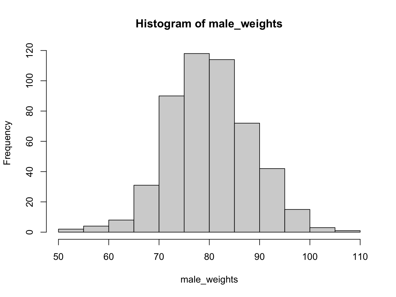
Using the breaks argument, you can adjust the bin width. Always explore this option when creating histograms!
par(mfrow = c(1, 2)) # make 2 plots to sit side by side
hist(male_weights, breaks = 5, col = "gold", main = "Male weights")
hist(male_weights, breaks = 25, col = "green", main = "Male weights")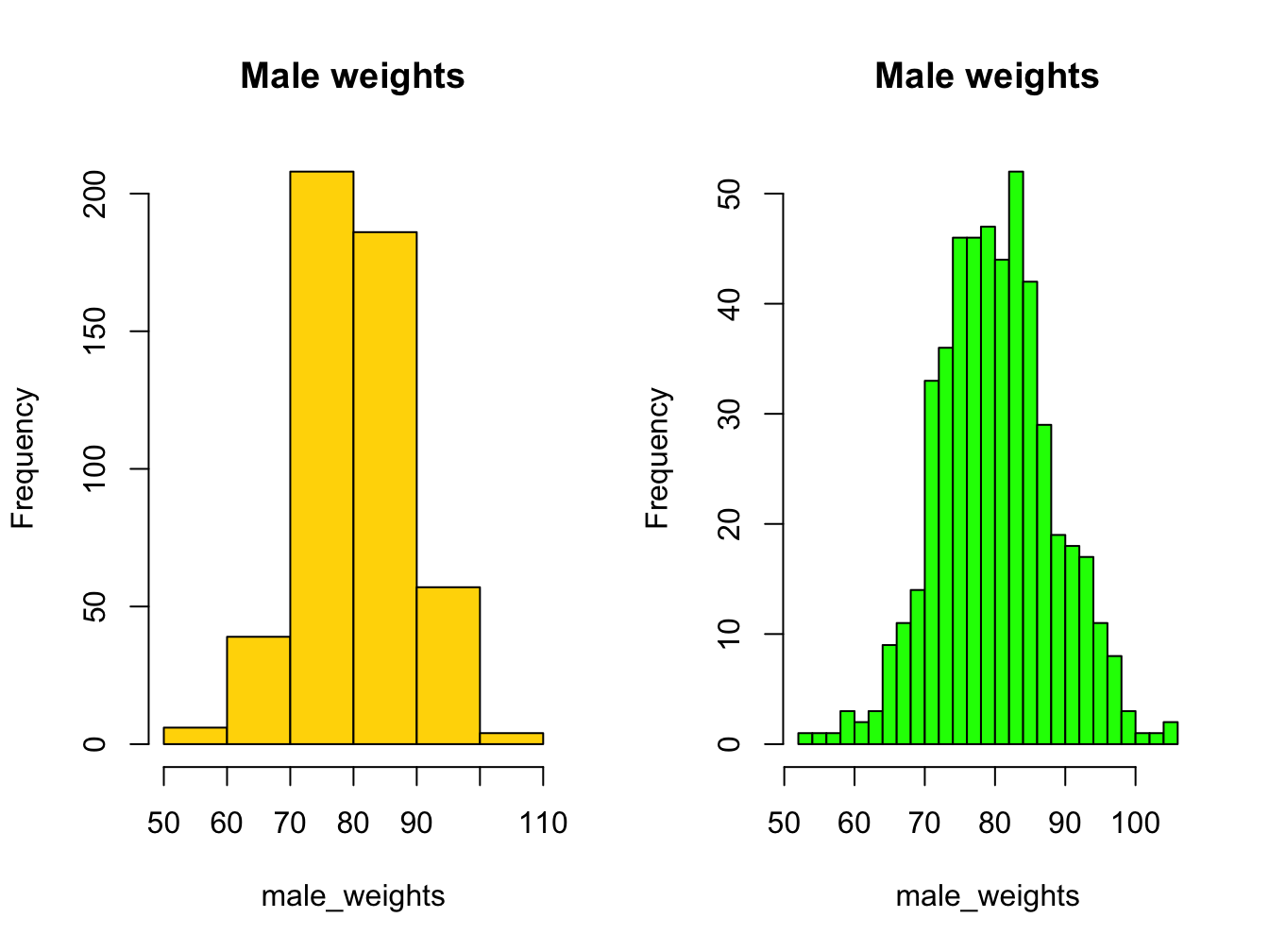
If you want a more detailed
3.2.4 Density plot as alternative to hist()
When you want a bit more fine-grained view of the distribution you can use a plot of a density function; by adding a polygon() you can even have some nice shading under the line:
plot(density(male_weights),
     main = "A density plot of male weights",
     col = "blue", lwd = 2)
polygon(density(male_weights), col="lightblue")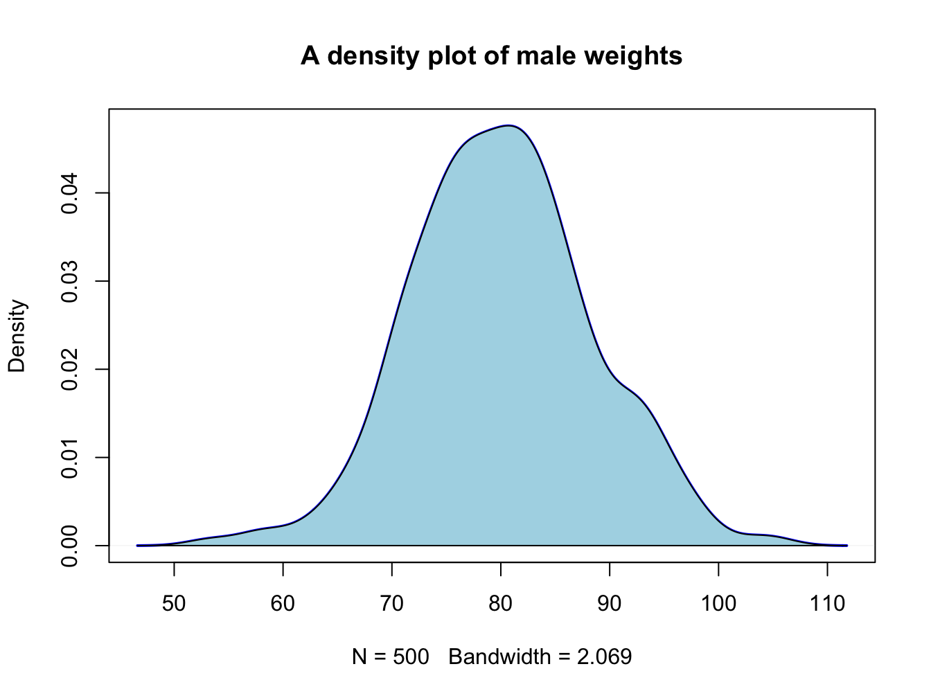
3.2.5 Boxplots
This is the last of the basic plot types. A boxplot is a visual representation of the 5-number summary of a numeric variable: minimum, maximum, median, first and third quartile.
persons <- rep(c("male", "female"), each = 100)
weights <- c(rnorm(100, 80, 6), rnorm(100, 75, 8))
#print 6-number summary (5-number + mean)
summary(weights[persons == "female"])
## Min. 1st Qu. Median Mean 3rd Qu. Max.
## 57.68 69.36 74.12 73.99 78.97 92.23Boxplots tell the same story as histograms, but are less precise. however, they are excellent when you want to show a series of subsets split over some variable.
par(mfrow = c(1, 2)) # make 2 plots to sit side by side
# create boxplots of weights depending on sex
boxplot(weights ~ persons, ylab = "weight")
boxplot(weights ~ persons, notch = TRUE, col = c("yellow", "magenta"))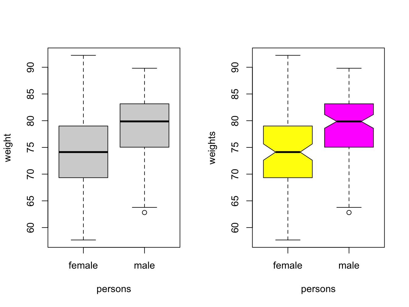
Use varwidth = TRUE when you want to visualize the difference in group sizes.
3.2.6 Adding more data and a legend
When you have more than one data series to plot, add them using the function points(). You call this function after you created the primary plot. Since there are multiple lines you will also need a legend.
response2 <- c(0.07, 0.10, 0.17, 0.28, 0.46, 0.61)
plot(x = time, y = response, pch = 19, type = "b",
     xlab = "Time (hours)", ylab = "Systemic response (a.u.)",
     main = "Systemic response to agent X", col = "blue")
points(x = time, y = response2, col = "red", pch = 19, type = "b")
legend(x = 1, y = 1.0, legend = c("one", "two"), col = c("blue", "red"), pch = 19)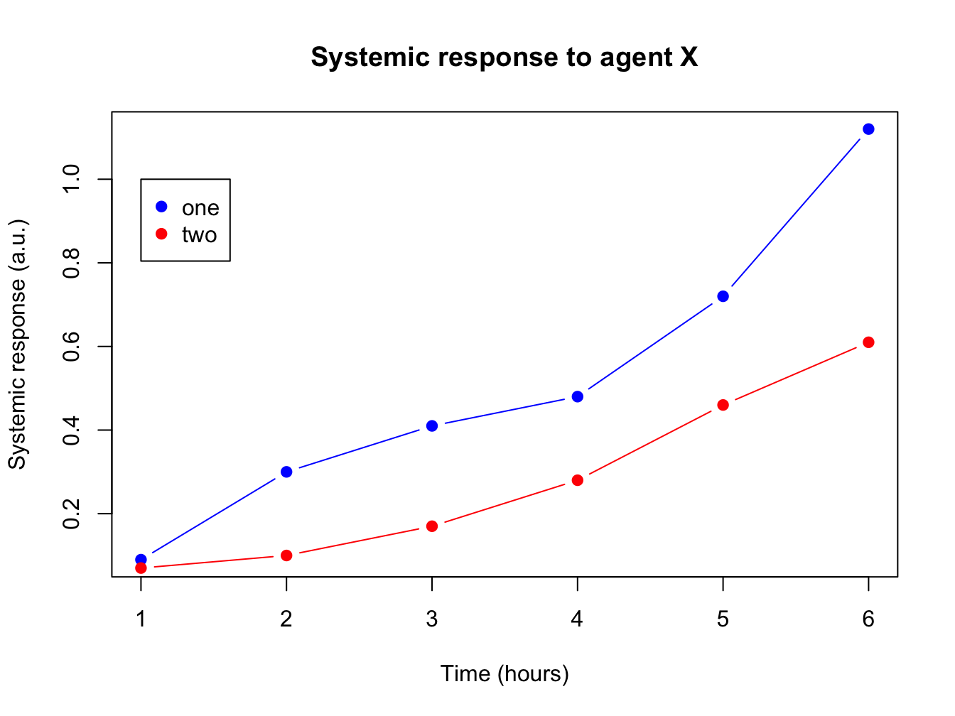
The legend() function is very versatile. Have a look at the docs!
In its most basic form you pass it a position (x and y), series names, colors and plot character.
3.2.7 Helper lines and lm()
Adding helper lines can be used to aid your reader in grasping and interpreting your data story.
Use the function abline() for this.
There are four types of helper lines you might want to add to a figure:
- A horizontal line with
h =: indicate some y-threshold - A vertical line with
v =: indicate x-threshold or mean or some other statistic - A line with an intercept (
a =) and a slope (b =): often used to indicate some expected response, or diagonal x = y - A linear model, determined with the
lm()function. The linear model object actually contains an intercept and a slope value which is taken byabline().
In the following plot, these four basic helper lines are demonstrated:
plot(x = time, y = response, pch = 19, type = "b",
     xlab = "Time (hours)", ylab = "Systemic response (a.u.)",
     main = "Systemic response to agent X", col = "blue")
#horizontal line
abline(h = 0.3, lty = 2, lwd = 2, col = "red")
#vertical line
abline(v = 4, lty = 3, lwd = 2, col = "darkgreen")
#line with slope
abline(a = -0.1, b = 0.3, lwd = 2, col = "purple")
#linear model
abline(lm(response ~ time),  lwd = 2, col = "maroon")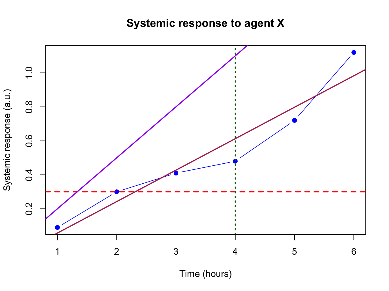
3.2.8 Graphical parameters to plot()
There are many parameters that can be passed to the plotting functions. Here is a small sample and their possible values.
series <- 1:20
plot(0, 0, xlim=c(1,20) , ylim=c(0.5, 7.5), col="white" , yaxt="n" , ylab="" , xlab="")

# the rainbow() function gives a nice palette across all colors
# or use hcl.colors() to specify another palette
# use  hcl.pals() to get an overview of available pallettes
colors = hcl.colors(20, alpha = 0.8, palette = 'viridis')

#pch
points(series, rep(1, 20), pch = 1:20, cex = 2)
#col
points(series, rep(2, 20), col = colors, pch = 16, cex = 3)
#cex
points(series, rep(3, 20), col = "black" , pch = 16, cex = series * 0.2)

#overlay to create new symbol
points(series, rep(4, 20), pch = series, cex = 2.5, col = "blue")
points(series, rep(4, 20), pch = series, cex = 1.5, col = colors)

#lty
for (i in 1:6) {
    points(c(-2, 0) + (i * 3), c(5, 5), col = "black", lty = i, type = "l", lwd = 3)
    text((i * 3) - 1, 5.25 , i)
}
#type and lwd
for (i in 1:4) {
    #type
    points(c(-4, -3, -2, -1) + (i * 5), rep(6, 4),
           col = "black", type = c("p","l","b","o")[i], lwd=2)
    text((i * 5) - 2.5, 6.4 , c("p","l","b","o")[i] )
    #lwd
    points(c(-4, -3, -2, -1) + (i * 5), rep(7, 4), col = "blue", type = "l", lwd = i)
    text((i * 5) - 2.5, 7.23, i)
}
#add axis
axis(side = 2, at = c(1, 2, 3, 4, 5, 6, 7),
    labels = c("pch" , "col" , "cex" , "combine", "lty", "type" , "lwd" ),
    tick = FALSE, col = "black", las = 1, cex.axis = 0.8)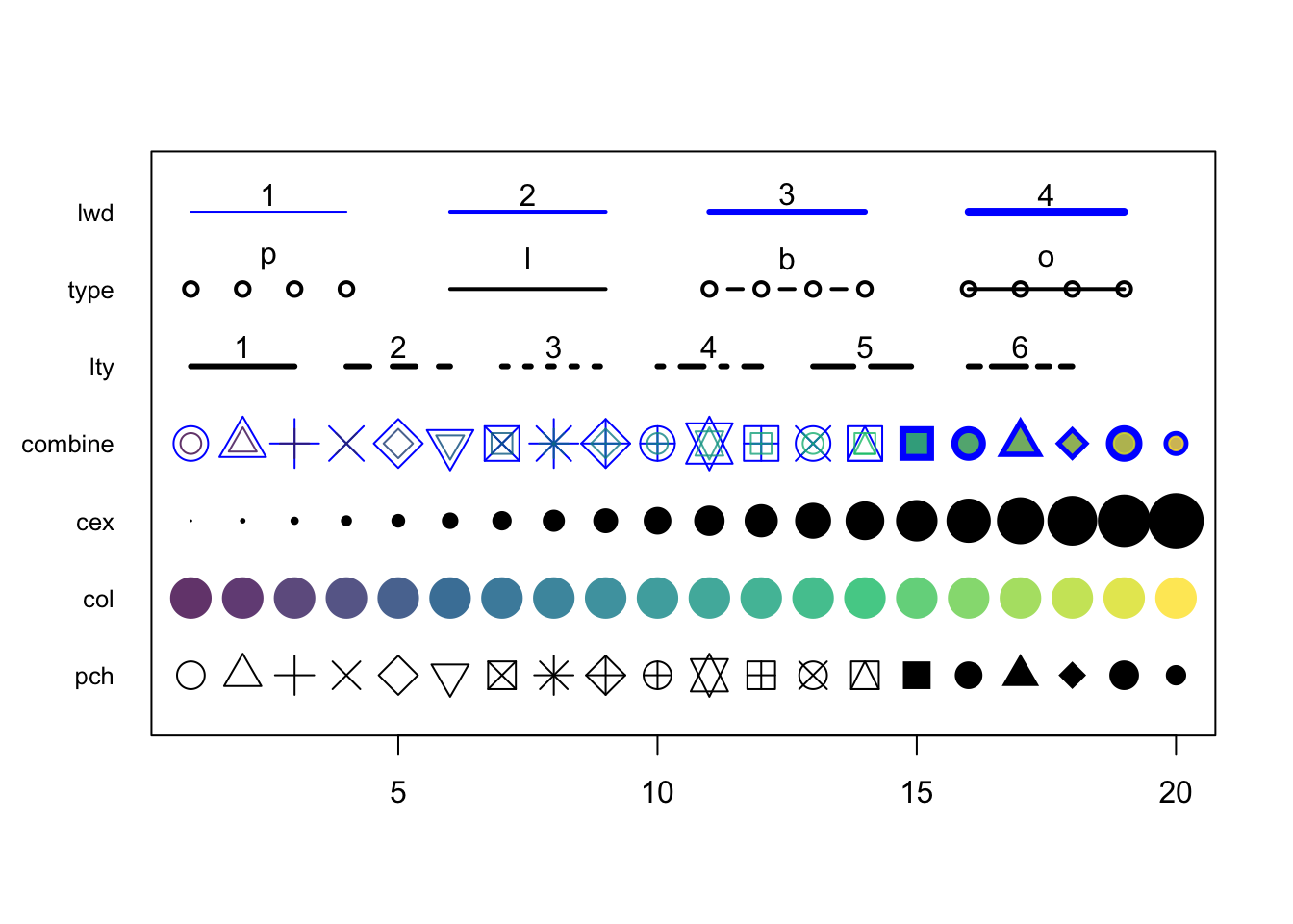
Comments
Everything on a line after a hash sign “
#” will be ignored by R. Use it to add explanation to your code: