9 Old school data mangling
This chapter deals with old-school data mangling using base R functions. These are presented for completeness’ sake, and also because sometimes these functions are simply the most convenient compared to what dplyr has to offer.
Dataframes are ubiquitous in R-based data analyses. Many R functions and packages are tailored specifically for DF manipulations - you have already seen cbind(), rbind() and subset().
In this presentation, we’ll explore a few new functions and techniques for working with DFs:
9.1 The apply() family of functions
Looping with for may be tempting, but highly discouraged in R because its inefficient. Usually one of these functions will do it better (or of course the dplyr functions discussed below):
-
apply: Apply a function over the “margins” of a dataframe - rows or columns or both -
lapply: Loop over a list and evaluate a function on each element; returns a list of the same length -
sapply: Same as lapply but try to simplify the result -
tapply: Apply a function over subsets of a vector (read: split with a factor)
There are more but these are the important ones.
9.1.0.1 apply(): Apply Functions Over Array Margins
- Suppose you want to know the means of all columns of a dataframe.
-
apply()needs to know- what DF to apply to (
X) - over which margin(s) - columns and/or rows (
MARGIN) - what function to apply (
FUN)
- what DF to apply to (
apply(X = cars, MARGIN = 2, FUN = mean) # apply over columns## speed dist
## 15.4 43.0Here, a function is applied to both columns and rows
df <- data.frame(x = 1:5, y = 6:10)
minus_one_squared <- function(x) (x-1)^2
apply(X = df, MARGIN = c(1,2), FUN = minus_one_squared)
## x y
## [1,] 0 25
## [2,] 1 36
## [3,] 4 49
## [4,] 9 64
## [5,] 16 81(Ok, that was a bit lame: minus_one_squared(df) does the same)
The Body Mass Index, or BMI, is calculated as \((weight / height ^ 2) * 703\) where weight is in pounds and height in inches. Here it is calculated for the build in dataset women.
head(women, n=3)## height weight
## 1 58 115
## 2 59 117
## 3 60 120## height weight bmi
## 1 58 115 24.0
## 2 59 117 23.6
## 3 60 120 23.4
## 4 61 123 23.2Pass arguments to the applied function
Sometimes the applied function needs to have other arguments passed besides the row or column. The ... argument to apply() makes this possible (type ?apply to see more info)
# function sums and powers up
spwr <- function(x, p = 2) {sum(x)^p}
# a simple dataframe
df <- data.frame(a = 1:5, b = 6:10)
df
## a b
## 1 1 6
## 2 2 7
## 3 3 8
## 4 4 9
## 5 5 10
# spwr will use the default value for p (p = 2)
apply(X = df, MARGIN = 1, FUN = spwr)
## [1] 49 81 121 169 225
# pass power p = 3 to function spwr (argument names omitted)
apply(df, 1, spwr, p = 3)
## [1] 343 729 1331 2197 3375Note: The ... argument works for all ..apply.. functions.
9.1.0.2 lapply(): Apply a Function over a List or Vector
Function lapply() applies a function to all elements of a list and returns a list with the same length, each element the result of applying the function
myNumbers = list(
    one = c(1, 3, 4),
    two = c(3, 2, 6, 1),
    three = c(5, 7, 6, 8, 9))
lapply(X = myNumbers, FUN = mean)
## $one
## [1] 2.67
##
## $two
## [1] 3
##
## $three
## [1] 7Here is the same list, but now with sqrt() applied. Notice how the nature of the applied function influences the result.
lapply(X = myNumbers, FUN = sqrt)## $one
## [1] 1.00 1.73 2.00
##
## $two
## [1] 1.73 1.41 2.45 1.00
##
## $three
## [1] 2.24 2.65 2.45 2.83 3.00
9.1.0.3 sapply(): Apply a Function over a List or Vector and Simplify
When using the same example as above, but with sapply, you get a vector returned. Note that the resulting vector is a named vector, a convenient feature of sapply
myNumbers = list(
    one = c(1, 3, 4),
    two = c(3, 2, 6, 1),
    three = c(5, 7, 6, 8, 9))
sapply(X = myNumbers, FUN = mean)
## one two three
## 2.67 3.00 7.00When the result can not be simplified, you get the same list as with lapply():
sapply(X = myNumbers, FUN = sqrt)## $one
## [1] 1.00 1.73 2.00
##
## $two
## [1] 1.73 1.41 2.45 1.00
##
## $three
## [1] 2.24 2.65 2.45 2.83 3.009.1.0.4 wasn’t a dataframe also a list?
Yes! It is also list(ish). Both lapply() and sapply() work just fine on dataframes:
lapply(X = cars, FUN = mean)## $speed
## [1] 15.4
##
## $dist
## [1] 43
sapply(X = cars, FUN = mean) ## speed dist
## 15.4 43.0By the way, sapply and lapply also work with vectors.
9.1.0.5 tapply(): Apply a Function Over a Ragged Array
What tapply() does is apply a function over subsets of a vector; it splits a vector into groups according to the levels in a second vector and applies the given function to each group.
tapply(X = chickwts$weight, INDEX = chickwts$feed, FUN = sd)## casein horsebean linseed meatmeal soybean sunflower
## 64.4 38.6 52.2 64.9 54.1 48.89.2 Other data mangling functions
9.2.0.1 split(): Divide into Groups and Reassemble
This is similar to tapply() in the sense that is uses a factor to split its first argument. But where tapply() splits a vector, split() splits a dataframe - into list of dataframes.
You use split() when a dataframe needs to be divided depending on the value of some grouping variable.
Here we have the response of Treated (T) and Untreated (UT) subjects
myData <- data.frame(
    response = c(5, 8, 4, 5, 9, 3, 6, 7, 3, 6, 5, 2),
    treatment = factor(
        c("UT", "T", "UT", "UT", "T", "UT", "T", "T", "UT", "T", "T", "UT")))
splData <- split(x = myData, f = myData$treatment)
str(splData)
## List of 2
## $ T :'data.frame': 6 obs. of 2 variables:
## ..$ response : num [1:6] 8 9 6 7 6 5
## ..$ treatment: Factor w/ 2 levels "T","UT": 1 1 1 1 1 1
## $ UT:'data.frame': 6 obs. of 2 variables:
## ..$ response : num [1:6] 5 4 5 3 3 2
## ..$ treatment: Factor w/ 2 levels "T","UT": 2 2 2 2 2 2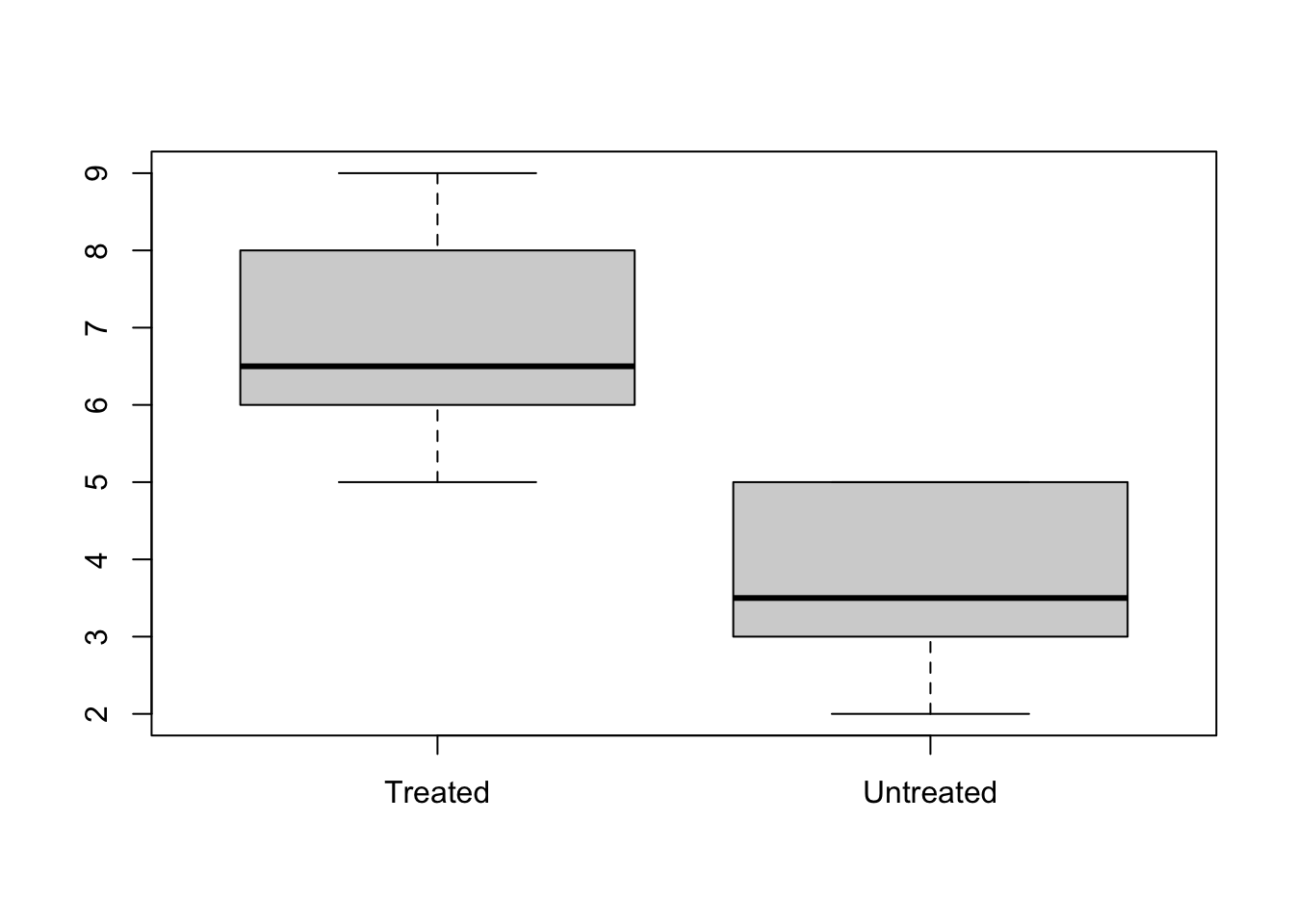
Note that this trivial example could also have been done with boxplot(myData$response ~ myData$treatment).
Here you can see that split() also works with vectors.
## $healthy
## [1] -1.4482  0.5748 -1.0237 -0.0151 -0.9359
##
## $sick
## [1]  0.134 -0.491 -0.441  0.460 -0.694
9.2.0.2 aggregate(): Compute Summary Statistics of Data Subsets
Splits the data into subsets, computes summary statistics for each, and returns the result in a convenient form.
aggregate(Temp ~ Month,
          data = airquality,
          FUN = mean)
## Month Temp
## 1 May 65.5
## 2 June 79.1
## 3 July 83.9
## 4 August 84.0
## 5 September 76.9Aggregate has two usage techniques:
with a formula:
aggregate(formula, data, FUN, ...)with a list:
aggregate(x, by, FUN, ...)
I really like aggregate(), especially the first form. That is, until I got to know the dplyr package.
Both forms of aggregate() will be demonstrated
Aggregate with formula
The left part of the formula accepts one, several or all columns as dependent variables.
##       Month Temp Ozone
## 1       May 66.7  23.6
## 2      June 78.2  29.4
## 3      July 83.9  59.1
## 4    August 84.0  60.0
## 5 September 76.9  31.4
##all
aggregate(. ~ Month,
          data = airquality,
          FUN = mean)
## Month Ozone Solar.R Wind Temp Day bar
## 1 May 24.1 182 11.50 66.5 16.1 0.333
## 2 June 29.4 184 12.18 78.2 14.3 0.333
## 3 July 59.1 216 8.52 83.9 16.2 0.808
## 4 August 60.0 173 8.86 83.7 17.2 0.696
## 5 September 31.4 168 10.08 76.9 15.1 0.345The right part can also accept multiple independent variables
airquality$Temp_factor <- cut(airquality$Temp,
                              breaks = 2,
                              labels = c("low", "high"))
aggregate(Ozone ~ Month + Temp_factor,
          data = airquality,
          FUN = mean)
## Month Temp_factor Ozone
## 1 May low 18.9
## 2 June low 20.5
## 3 July low 13.0
## 4 August low 16.0
## 5 September low 17.6
## 6 May high 80.0
## 7 June high 36.6
## 8 July high 63.0
## 9 August high 63.6
## 10 September high 48.5The by = list(...) form
This is the other form of aggregate. It is more elaborate in my opinion because you need te spell out all vectors you want to work on.
##        feed   x
## 1    casein 324
## 2 horsebean 160
## 3   linseed 219
## 4  meatmeal 277
## 5   soybean 246
## 6 sunflower 329
Here is another example:
aggregate(x = airquality$Wind,
          by = list(month = airquality$Month, temperature = airquality$Temp_factor),
          FUN = mean)
## month temperature x
## 1 May low 11.71
## 2 June low 9.85
## 3 July low 10.60
## 4 August low 11.43
## 5 September low 11.39
## 6 May high 10.30
## 7 June high 10.51
## 8 July high 8.83
## 9 August high 8.51
## 10 September high 8.79But it is better to wrap it in with():
9.2.1 Many roads lead to Rome
The next series of examples are all essentially the same. The message is: there is more than one way to do it!
aggregate(weight ~ feed,
          data = chickwts,
          FUN = mean)
## feed weight
## 1 casein 324
## 2 horsebean 160
## 3 linseed 219
## 4 meatmeal 277
## 5 soybean 246
## 6 sunflower 329same as
##        feed   x
## 1    casein 324
## 2 horsebean 160
## 3   linseed 219
same as
tapply(chickwts$weight, chickwts$feed, mean)## casein horsebean linseed meatmeal soybean sunflower
## 324 160 219 277 246 329## casein horsebean linseed meatmeal soybean sunflower
## 324 160 219 277 246 329same as
##    casein horsebean   linseed  meatmeal   soybean sunflower
## 324 160 219 277 246 329And this is the topic of the next part of this chapter:
## # A tibble: 6 × 2
##   feed      mean_weigth
##   <fct>           <dbl>
## 1 casein           324.
## 2 horsebean        160.
## 3 linseed          219.
## 4 meatmeal         277.
## 5 soybean          246.
## 6 sunflower        329.