14 Exploratory Data Analysis I

14.1 Introduction

This chapter introduces you to the concept of Exploratory Data Analysis (EDA). The purpose of an EDA is analysing a dataset with the goal of assessing its main characteristics, including quality and usability for subsequent statistical modelling and analysis. Data cleaning and transformation strategies are explored and often already applied. Data summary techniques and visualizations are used in an EDA. There is no fixed set of activities; each dataset poses its own questions and challenges.

Datasets are often expensive and time-consuming to collect, and therefore they are usually collected with a specific goal in mind. The EDA you perform should always be with this goal in mind: is the dataset of sufficient quality to answer the scientific questions for which they were collected?

The current EDA is the first of two; this one mainly uses base R functionality (except for plotting where ggplot2 is used) while the next one mainly employs tidyverse functionality.

EDA outline

An EDA therefore may include:

Dataset description: how were they collected, what data types do the variables have, what are the units and physical quantities, how are missing data encoded, etc.
Data summary: number of cases, number of variables, basic statistical description (i.e. mean, median, sd etc.), variable distributions (normal or not, outliers, missing data, skewed distributions)
Visual summaries using boxplots, histograms, density plots.
Recoding or transformations of variables may be required to get better results (e.g. from numeric to factor or vice versa, or log transformation of exponential data)
Exploration of variable relations/covariance. It is always interesting to know about correlations between variables, but this is especially the case when you have a dependent variable for which you wish to build a statistical model in a later stage of your analysis.

Note that your EDA results should always be accompanied by text that describes your results and discusses the implications of them. your figures should be well annotated with a caption and legend if relevant. An EDA is not a publication, but it will usually have a short introduction, a results section and a discussion. In contrast with a publication you usually do show the code. This ensures complete transparency and reproducibility.

In this chapter I will demonstrate a short EDA on the “Yeast dataset” from the UCI Machine Learning repository.

It is outside the scope of this short analysis to delve too deeply in the attribute background information, but you should realize that for a real analysis this is absolutely critical: without domain knowledge the you won’t have the insight to identify strange, worrying or surprising results.

14.2 EDA of the Yeast dataset

14.2.1 Introduction

The data were collected from the UCI Machine Learning website. To ensure their continued availability the files were copied to a personal repository.

The data were accompanied by a very short abstract: “Predicting the Cellular Localization Sites of Proteins”. The data description states there are 1484 instances, each with 8 attributes (variables) and a class label. The class label is the variable we wish to build a model for so this is the dependent variable.

The Attribute Information section describes these variables:

Sequence Name: Accession number for the SWISS-PROT database
mcg: McGeoch’s method for signal sequence recognition.
gvh: von Heijne’s method for signal sequence recognition.
alm: Score of the ALOM membrane spanning region prediction program.
mit: Score of discriminant analysis of the amino acid content of the N-terminal region (20 residues long) of mitochondrial and non-mitochondrial proteins.
erl: Presence of “HDEL” substring (thought to act as a signal for retention in the endoplasmic reticulum lumen). Binary attribute.
pox: Peroxisomal targeting signal in the C-terminus.
vac: Score of discriminant analysis of the amino acid content of vacuolar and extracellular proteins.
nuc: Score of discriminant analysis of nuclear localization signals of nuclear and non-nuclear proteins.

The sequence name is not interesting in this EDA: we are interested in patterns, not individuals. However, if there is an anomalous protein in the EDA it should be possible to retrace its origin so the identifier stays in the dataset.

There seem to be two attributes (mcg and gvh) measuring the same property - the presence of a signal sequence which is the N-terminal part of a protein signalling the cellular machinery the protein should be exported.

Very simply put, if this scoring system was perfect each of the attributes (except mcg and gvh) would unequivocally “assign” the protein in question to a cellular location: Cellular external matrix, membrane inserted, mitochondrial, endoplasmic reticulum lumen, peroxisomal, vacuolar or nuclear.

The tenth variable in the data is the dependent or explanatory variable. The yeast.names file describes it like this:

Class Distribution. The class is the localization site. Please see Nakai &
               Kanehisa referenced above for more details.
  CYT (cytosolic or cytoskeletal)                    463
  NUC (nuclear)                                      429
  MIT (mitochondrial)                                244
  ME3 (membrane protein, no N-terminal signal)       163
  ME2 (membrane protein, uncleaved signal)            51
  ME1 (membrane protein, cleaved signal)              44
  EXC (extracellular)                                 37
  VAC (vacuolar)                                      30
  POX (peroxisomal)                                   20
  ERL (endoplasmic reticulum lumen)                    5

This tells me the different localizations are by no means equally distributed; there is an over representation of “cytosolic or cytoskeletal” and “nuclear” and a huge under representation of especially endoplasmic reticulum lumen proteins.

14.2.2 Data loading and prepping

Since I am going to rerun the code in this notebook often I am going to create a local copy, and load that one.

file_name <- "yeast.data"
yeast_data_url <- paste0("https://raw.githubusercontent.com/MichielNoback/datasets/master/UCI_yeast_protein_loc/", file_name)
yeast_local_location <- paste0("./data/", file_name)

#only download if not present
if (! file.exists(yeast_local_location)) {
    download.file(url = yeast_data_url, 
                  destfile = yeast_local_location)
}

yeast_data <- read.table(file = yeast_local_location,
                         sep = ",",
                         as.is = 1)
str(yeast_data)

## 'data.frame':    1484 obs. of  10 variables:
##  $ V1 : chr  "ADT1_YEAST" "ADT2_YEAST" "ADT3_YEAST" "AAR2_YEAST" ...
##  $ V2 : num  0.58 0.43 0.64 0.58 0.42 0.51 0.5 0.48 0.55 0.4 ...
##  $ V3 : num  0.61 0.67 0.62 0.44 0.44 0.4 0.54 0.45 0.5 0.39 ...
##  $ V4 : num  0.47 0.48 0.49 0.57 0.48 0.56 0.48 0.59 0.66 0.6 ...
##  $ V5 : num  0.13 0.27 0.15 0.13 0.54 0.17 0.65 0.2 0.36 0.15 ...
##  $ V6 : num  0.5 0.5 0.5 0.5 0.5 0.5 0.5 0.5 0.5 0.5 ...
##  $ V7 : num  0 0 0 0 0 0.5 0 0 0 0 ...
##  $ V8 : num  0.48 0.53 0.53 0.54 0.48 0.49 0.53 0.58 0.49 0.58 ...
##  $ V9 : num  0.22 0.22 0.22 0.22 0.22 0.22 0.22 0.34 0.22 0.3 ...
##  $ V10: Factor w/ 10 levels "CYT","ERL","EXC",..: 7 7 7 8 7 1 7 8 7 1 ...

The data seems to have been loaded correctly and, as expected since that was stated in the original data description, there are no missing data.

The column names were not defined in the data file so this will be fixed first. I will create a data frame that also holds the column descriptions. I have put the data in a small text file for easy loading and editing; the attribute descriptions copied/pasted into a text file and with find/replace converted in easy to load form, and a new label column added for use in plotting. There were a few occurrences of the ' character which always corrupt data import into R. They were removed.

attribute_info <- read.table("data/yeast_attribute_info.txt", 
                             sep = ":",
                             header = TRUE,
                             stringsAsFactors = FALSE)
#attach column names
(colnames(yeast_data) <- attribute_info$attribute)

##  [1] "accno" "mcg"   "gvh"   "alm"   "mit"   "erl"   "pox"   "vac"   "nuc"  
## [10] "loc"

To make this info easily accessible, a function is created that can be used to fetch either the description or the label.

get_attribute_info <- function(attribute, resource = "label") {
    if (! resource %in% c("label", "description")) {
        stop(paste0("type ", resource, "is not an attribute resource"))
    }
    return(attribute_info[attribute_info$attribute == attribute, resource])
}

#test it
get_attribute_info("gvh")
get_attribute_info("accno", "description")

## [1] "VonHeijne signal"
## [1] "Accession number for the SWISS-PROT database"

14.2.3 Data verification

The original data description stated that 1484 instances with 9 attributes + a class label are present.

dim(yeast_data)

## [1] 1484   10

This is correct. No missing data are supposed to be there:

sum(complete.cases(yeast_data))

## [1] 1484

Also correct.

The classes of the columns are also OK so the data is verified and found correct.

14.2.4 Attribute summaries

A first scan of the attributes.

summary(yeast_data)

##     accno                mcg            gvh            alm      
##  Length:1484        Min.   :0.11   Min.   :0.13   Min.   :0.21  
##  Class :character   1st Qu.:0.41   1st Qu.:0.42   1st Qu.:0.46  
##  Mode  :character   Median :0.49   Median :0.49   Median :0.51  
##                     Mean   :0.50   Mean   :0.50   Mean   :0.50  
##                     3rd Qu.:0.58   3rd Qu.:0.57   3rd Qu.:0.55  
##                     Max.   :1.00   Max.   :1.00   Max.   :1.00  
##                                                                 
##       mit             erl             pox             vac            nuc       
##  Min.   :0.000   Min.   :0.500   Min.   :0.000   Min.   :0.00   Min.   :0.000  
##  1st Qu.:0.170   1st Qu.:0.500   1st Qu.:0.000   1st Qu.:0.48   1st Qu.:0.220  
##  Median :0.220   Median :0.500   Median :0.000   Median :0.51   Median :0.220  
##  Mean   :0.261   Mean   :0.505   Mean   :0.007   Mean   :0.50   Mean   :0.276  
##  3rd Qu.:0.320   3rd Qu.:0.500   3rd Qu.:0.000   3rd Qu.:0.53   3rd Qu.:0.300  
##  Max.   :1.000   Max.   :1.000   Max.   :0.830   Max.   :0.73   Max.   :1.000  
##                                                                                
##       loc     
##  CYT    :463  
##  NUC    :429  
##  MIT    :244  
##  ME3    :163  
##  ME2    : 51  
##  ME1    : 44  
##  (Other): 90

All these attributes seem to be in the range zero to one, except of course for the localization attribute and the accession number. This is not surprising since these attributes are all probabilities. The class distribution corresponds with the published data.

The The pox (Peroxisomal) and erl ( ER-retention) attributes, seem to have a really strange distribution and should be investigated further.

Here are all the numeric attributes in a single panel. I chose histogram over boxplot or density plot because it is more fine-grained than boxplot and very easy to interpret.

# a list to store the plots
my_plots <- list()

names_to_plot <- colnames(yeast_data[2:9])
for (i in 1:length(names_to_plot)) {
    col_to_plot <- names_to_plot[i]
    plt <- ggplot(data = yeast_data,
                  mapping = aes(x = !!sym(col_to_plot))) +
        geom_histogram(bins = 30) +
        xlab(col_to_plot)
    my_plots[[i]] <- plt
}
grid.arrange(grobs = my_plots, nrow = 2)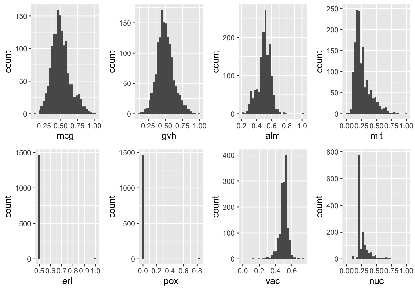

Figure 14.1: Distributions of the numeric variables

Here, it can be seen that the attributes “ER-retention” and “Peroxisomal” are pretty much uninformative, a problem probably largely caused by the low abundance of proteins in these classes. Surprisingly enough, the “Vacuolar” property which is also low-abundant, does not have this extreme distribution.

What is also striking is that, although these attributes are probabilities of targeting signals, none (with the exception of the two low-abundance ones) show a more or less bi-modal distribution as you would naively expect.

14.2.5 Attribute relationships

Here is a quick scan of variable relationship, excluding the dependent variable. The pairs() function is used for that. I excluded erl and pox because they do not add information to the picture.

# Function to return points and geom_smooth
# allow for the method to be changed
wrap_fn <- function(data, mapping, method="loess", ...){
      p <- ggplot(data = data, mapping = mapping) + 
      geom_point(size = 0.5, alpha = 0.4, color = "darkblue") + 
      geom_smooth(method=method, formula = 'y ~ x', ...)
      p
    }

ggpairs(yeast_data[c(2, 3, 4, 5, 8, 9)], 
        progress = FALSE,
        lower = list(continuous = wrap_fn))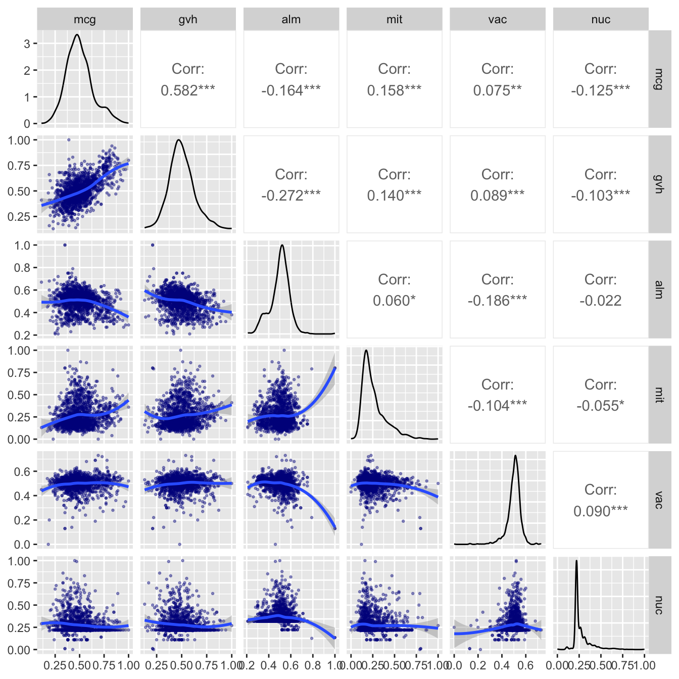

Figure 14.2: Relations between the numeric variables

NB: I found suggestions on how to adjust color, size etc here. If this is too complicated for you, you can simply use ggpairs(yeast_data[c(2, 3, 4, 5, 8, 9)], progress = FALSE)), or alternatively, base R has a nice pairs() function this creates a similar but less good looking plot.

By adding the smoother it is made clear that the only pair which shows a clear correlation is the pair mcg / gvh which actually predict the same property. Therefore it would have been very surprising indeed if they would not have a correlation. The strength of this correlation -the R-squared- is not very strong.

14.2.6 Correlations to the dependent variable

As a first investigation, numeric variables are split on the location variable. These plots are screated using the base R plotting system.

library(RColorBrewer)
colors <- RColorBrewer::brewer.pal(8, name = "Accent")
#col = c("darkblue", "darkgreen", "magenta", )
col_i <- 0
for (name in names(yeast_data[2:9])) {
    col_i <- col_i + 1
    boxplot(yeast_data[, name] ~ yeast_data$loc,
            xlab = NULL,
            ylab = get_attribute_info(name),
            col = colors[col_i])
}

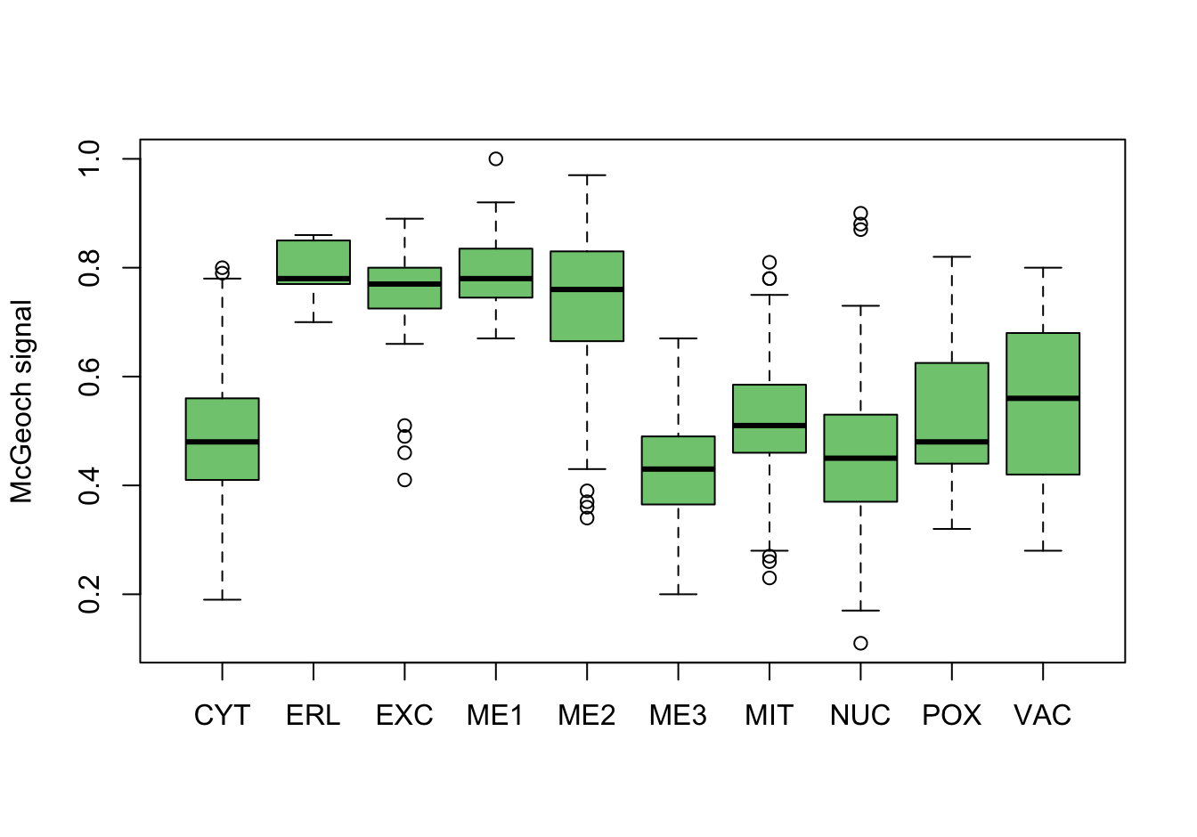
Figure 14.3: Correlations with the dependent variable

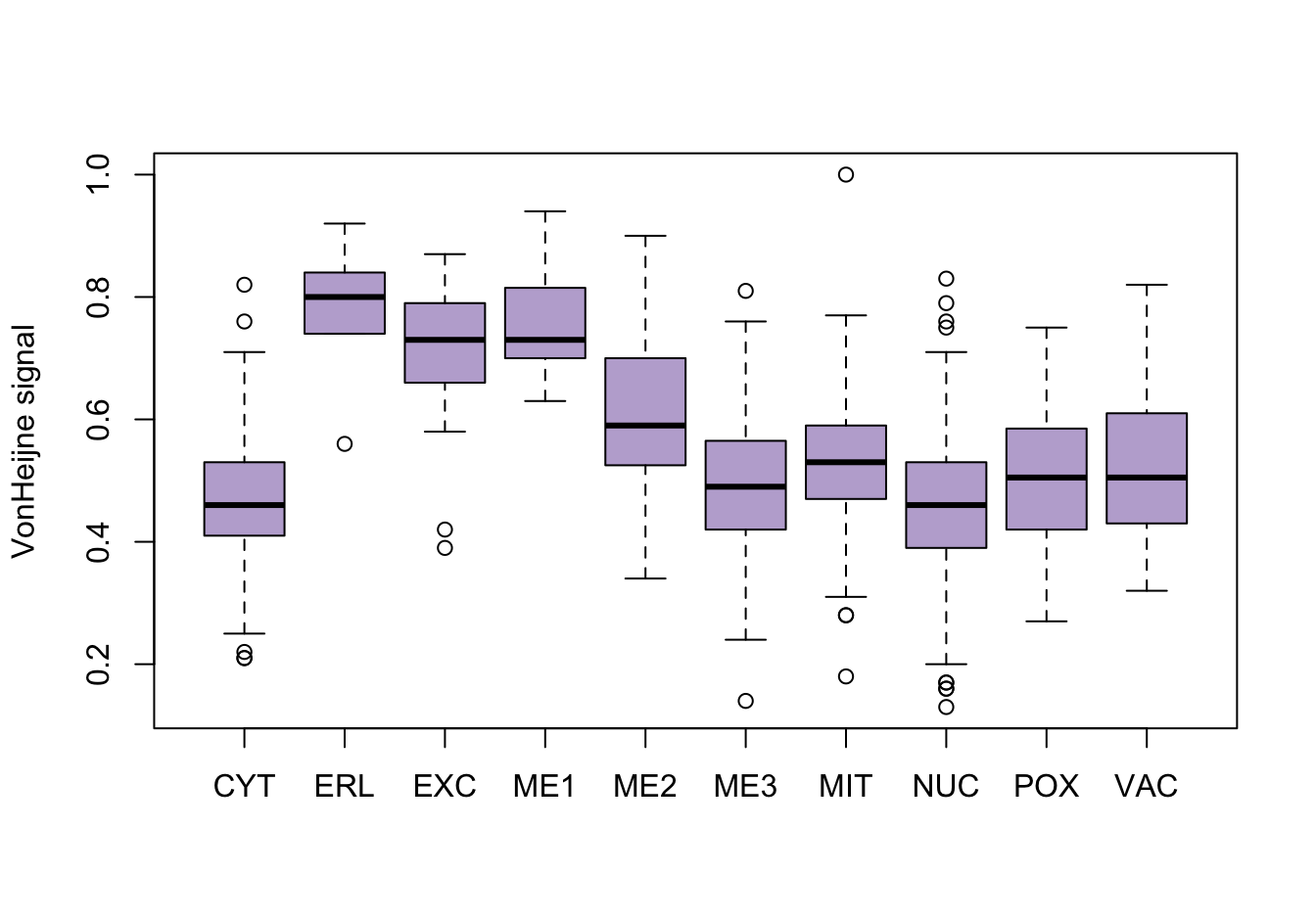
Figure 14.4: Correlations with the dependent variable

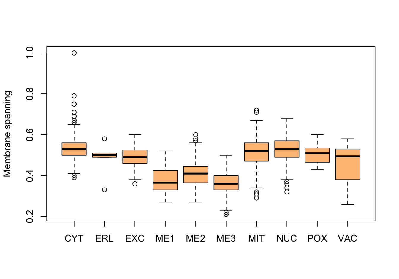
Figure 14.5: Correlations with the dependent variable

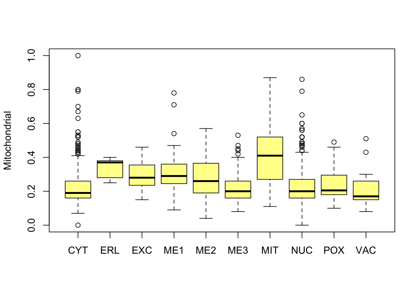
Figure 14.6: Correlations with the dependent variable

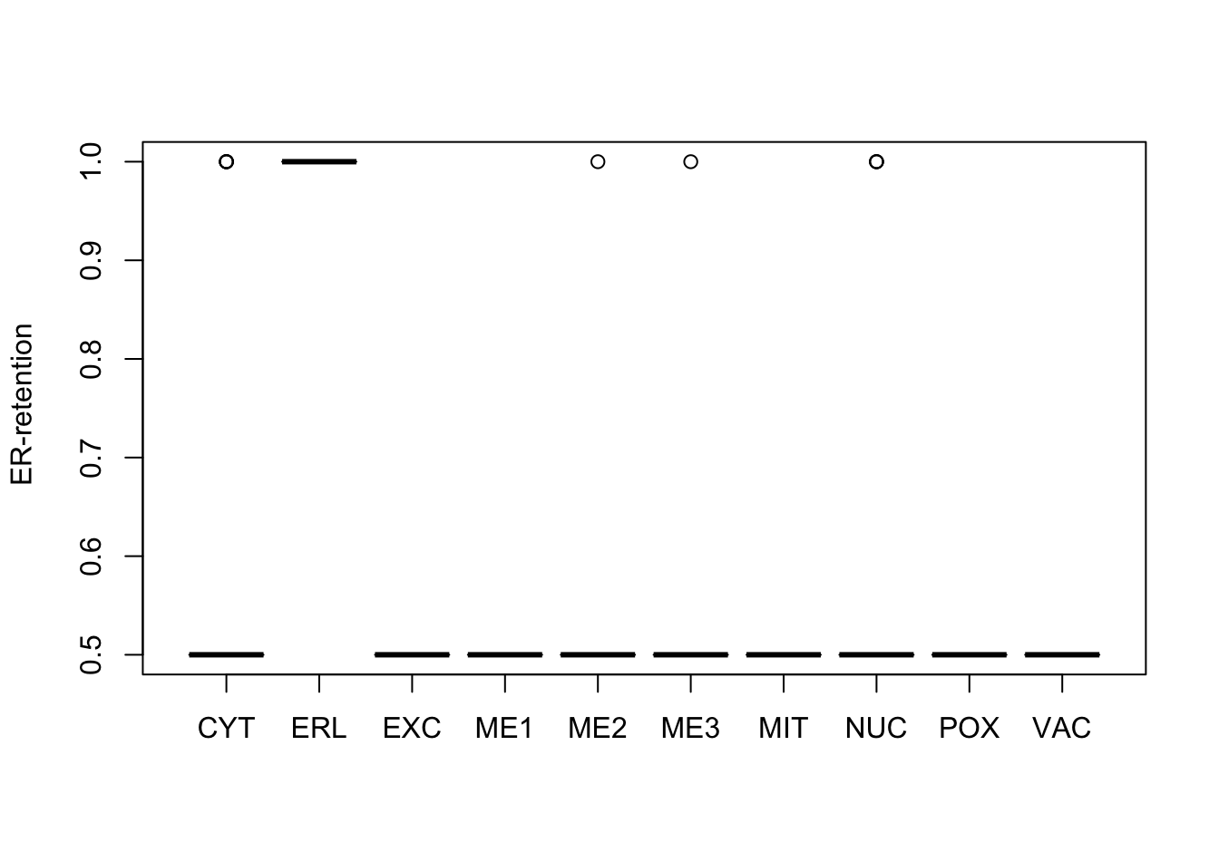
Figure 14.7: Correlations with the dependent variable

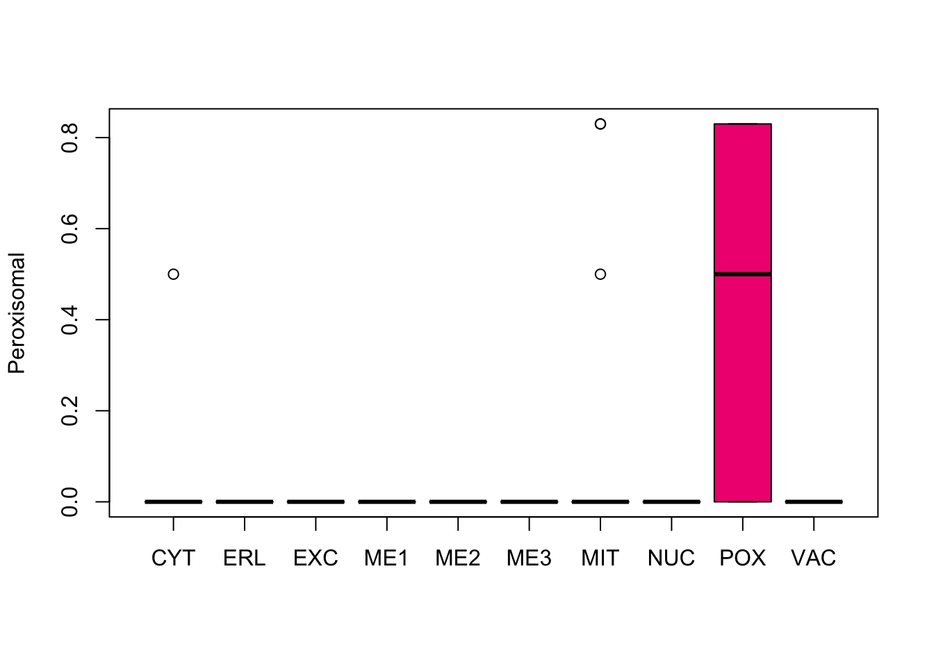
Figure 14.8: Correlations with the dependent variable

Figure 14.9: Correlations with the dependent variable

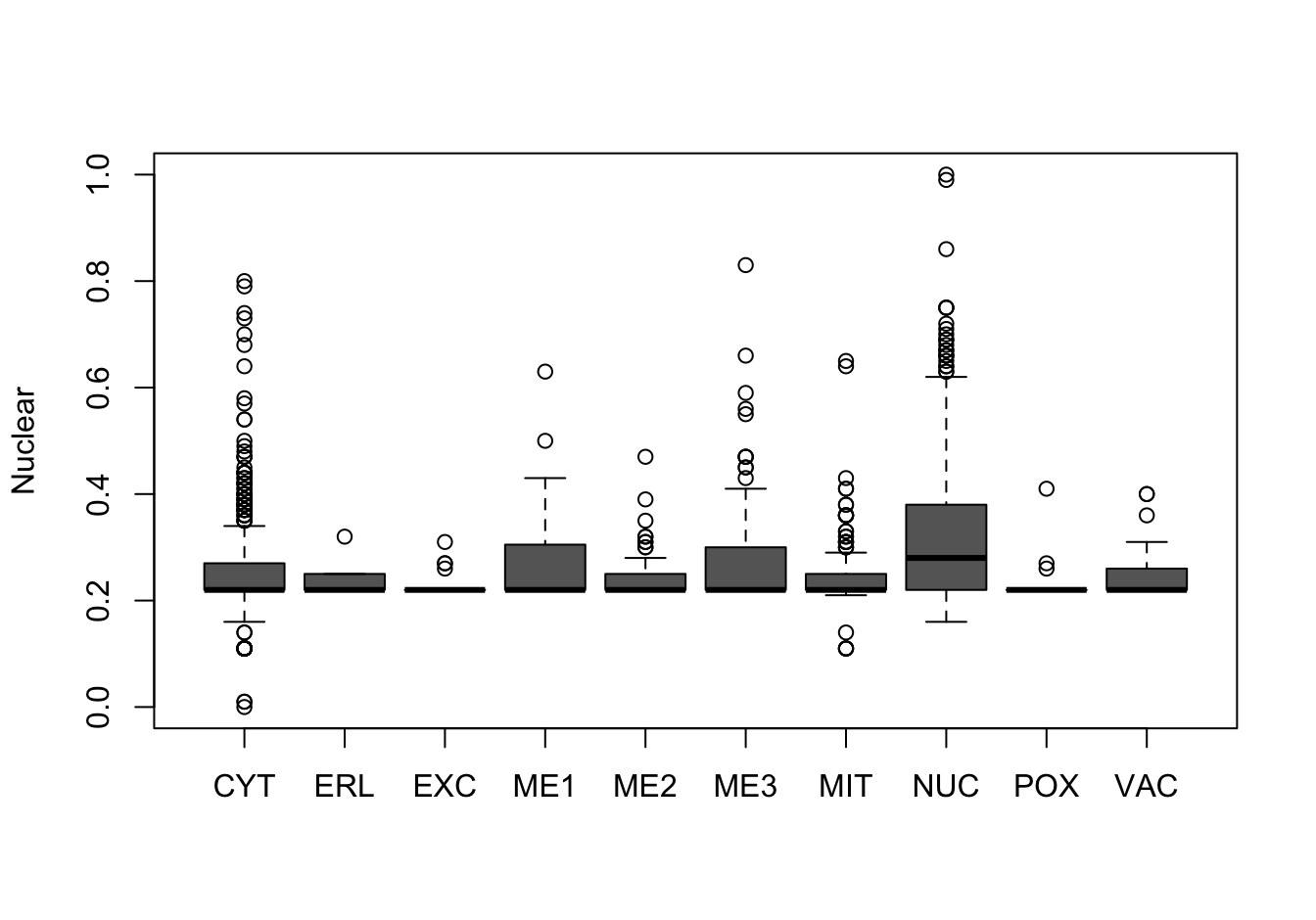
Figure 14.10: Correlations with the dependent variable

Quite a few of the variables correlate pretty well with the dependent variable. These do so very well: alm, mit, erl, pox. Others are not: nuc, vac, and some are ambiguous - they discriminate, but not exclusively: mcg, gvh.

Here are some summary statistics for the numeric variables split on the dependent variable:

options(digits=2)

tmp <- t(aggregate( . ~ loc, data = yeast_data[, -1], FUN = mean))
knitr::kable(tmp)

loc	CYT	ERL	EXC	ME1	ME2	ME3	MIT	NUC	POX	VAC
mcg	0.48	0.79	0.74	0.79	0.72	0.43	0.52	0.45	0.52	0.55
gvh	0.47	0.77	0.72	0.76	0.60	0.49	0.53	0.46	0.51	0.53
alm	0.54	0.48	0.49	0.38	0.41	0.36	0.52	0.53	0.51	0.47
mit	0.23	0.34	0.29	0.31	0.28	0.21	0.40	0.23	0.25	0.20
erl	0.50	1.00	0.50	0.50	0.51	0.50	0.50	0.50	0.50	0.50
pox	0.0011	0.0000	0.0000	0.0000	0.0000	0.0000	0.0089	0.0000	0.4235	0.0000
vac	0.50	0.55	0.46	0.51	0.51	0.51	0.50	0.49	0.50	0.53
nuc	0.26	0.25	0.23	0.27	0.25	0.27	0.24	0.33	0.23	0.25

tmp <- t(aggregate( . ~ loc, data = yeast_data[, -1], FUN = median))
knitr::kable(tmp)

loc	CYT	ERL	EXC	ME1	ME2	ME3	MIT	NUC	POX	VAC
mcg	0.48	0.78	0.77	0.78	0.76	0.43	0.51	0.45	0.48	0.56
gvh	0.46	0.80	0.73	0.73	0.59	0.49	0.53	0.46	0.51	0.51
alm	0.53	0.50	0.49	0.36	0.41	0.36	0.52	0.53	0.51	0.49
mit	0.19	0.37	0.28	0.29	0.26	0.20	0.41	0.20	0.21	0.17
erl	0.5	1.0	0.5	0.5	0.5	0.5	0.5	0.5	0.5	0.5
pox	0.0	0.0	0.0	0.0	0.0	0.0	0.0	0.0	0.5	0.0
vac	0.51	0.54	0.48	0.53	0.52	0.51	0.50	0.50	0.51	0.53
nuc	0.22	0.22	0.22	0.22	0.22	0.22	0.22	0.28	0.22	0.22

13 Working with date-time data

15 Exploratory Data Analysis II