6 Built-in Functions

This chapter deals with the most-used functions that R has to offer. A clean installation of R already contains hundreds of functions; see here for a complete listing of functions in the base package. Obviously, this eBook is not the platform to discuss these exhaustively. Therefore, I chose to only deal with the ones I use regularly.
Besides that, the tidyverse packages tidyr and dplyr offer functionality that are better alternatives for many base R functions. These packages are discussed in later chapters.

6.1 Descriptive statistics

R provides a wealth of descriptive statistics functions. The most important ones of them are listed below. The ones with an asterisk are described in more detail in following paragraphs.

function	purpose
`mean( )`	mean
`median( )`	median
`min( )`	minimum
`max( )`	maximum
`range( )`	min and max
`var( )`	variance s^2
`sd( )`	standard deviation s
`summary( )`	6-number summary
`quantile( )` *	quantiles
`IQR( )` *	interquantile range

The `quantile()` function

This function gives the data values corresponding to the specified quantiles. The function defaults to the quantiles 0% 25% 50% 75% 100%: these are the quartiles of course.

quantile(ChickWeight$weight)

##   0%  25%  50%  75% 100% 
##   35   63  103  164  373

quantile(ChickWeight$weight, probs = seq(0, 1, 0.2))

##   0%  20%  40%  60%  80% 100% 
##   35   57   85  126  182  373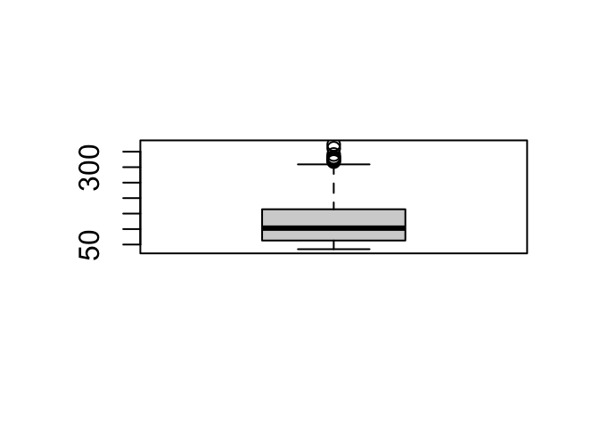

Interquantile range `IQR()`

Function IQR() gives the range between the 25% and 75% quantiles.

IQR(ChickWeight$weight)

## [1] 101

## same as
quantile(ChickWeight$weight)[4] - quantile(ChickWeight$weight)[2]

## 75% 
## 101

## same as
diff(quantile(ChickWeight$weight, probs = c(0.25, 0.75)))

## 75% 
## 101

`boxplot()` is `summary()` visualized

Boxplot is a graph of the 5-number summary, but summary() also gives the mean

summary(ChickWeight$weight)

##    Min. 1st Qu.  Median    Mean 3rd Qu.    Max. 
##      35      63     103     122     164     373

boxplot(ChickWeight$weight)

6.2 Sampling and distributions

You may have noticed the use of rnorm in a few examples of this book. This function samples values from a normal distribution. Sampling data from a distribution or specific collection of values is done very often. Here is a short overview of the main ones.

6.2.1 `rnorm` and friends.

Many distributions have been described in statistics. The most well-known is of course the normal distribution, characterized by the bell-shaped curve when a density plot is created.
Getting values from a normal distribution is done using the rnorm function. Actually, there is a family of related functions:

Density, distribution function, quantile function and random generation for the normal distribution with mean equal to mean and standard deviation equal to sd.

dnorm(x, mean = 0, sd = 1, log = FALSE)
pnorm(q, mean = 0, sd = 1, lower.tail = TRUE, log.p = FALSE)
qnorm(p, mean = 0, sd = 1, lower.tail = TRUE, log.p = FALSE)
rnorm(n, mean = 0, sd = 1)

where dnorm gives the density, pnorm gives the distribution function, qnorm gives the quantile function, and rnorm generates random deviates.
(see ?rnorm)

So, rnorm can be used to generate random values from a normal dstribution:

set.seed(4040)
random_normal <- rnorm(1000, 100, 8)

These values should give a nice bell-shaped curvee when plotted:

df <- data.frame(x = random_normal)
ggplot(data = df, mapping = aes(x = x)) +
    geom_histogram(aes(y = after_stat(density)), 
                   bins = 40, 
                   fill = "lightblue", 
                   color = "darkblue") +
    geom_density(color = "darkred", linewidth = 1.5)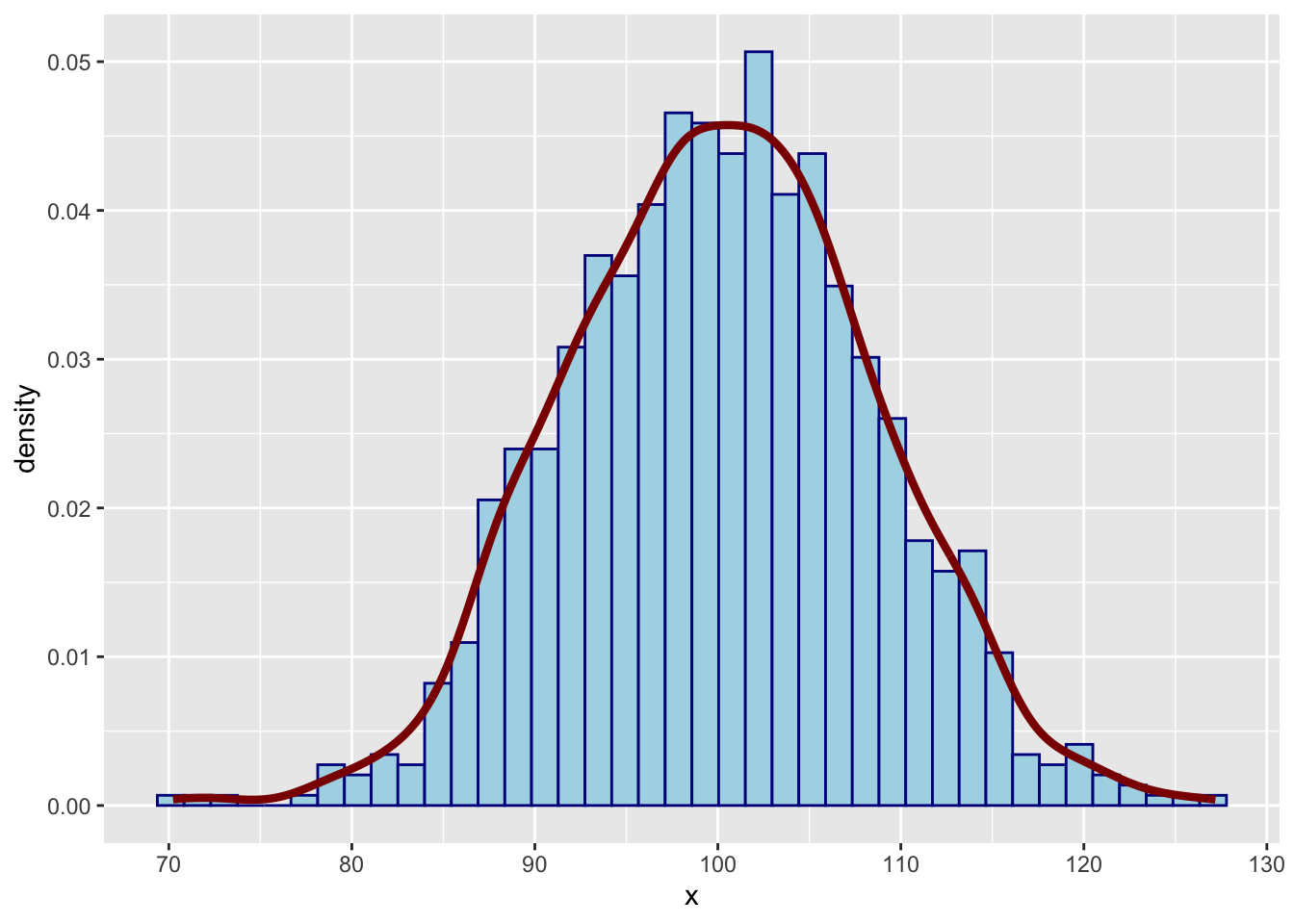

This is pretty close to a bell shape. You can check by adding a theoretical density function as well, using the dnorm function.

x <- seq(60, 130, length.out = 1000)
y_dens <- dnorm(x = x, mean = 100, sd = 8) # generate y values of theoretical density
df <- data.frame(x = x,
                obs = random_normal,
                y_dens = y_dens)
ggplot(data = df, mapping = aes(x = x)) +
    geom_histogram(aes(x = obs, y = after_stat(density)), 
                   bins = 40, 
                   fill = "lightblue",
                   color = "blue", 
                   alpha = 0.6) +
    geom_density(aes(x = obs), color = "darkred", linewidth = 1.3) + 
    geom_line(aes(y = y_dens), color = "darkgreen", linewidth = 1.3) +
    theme_minimal()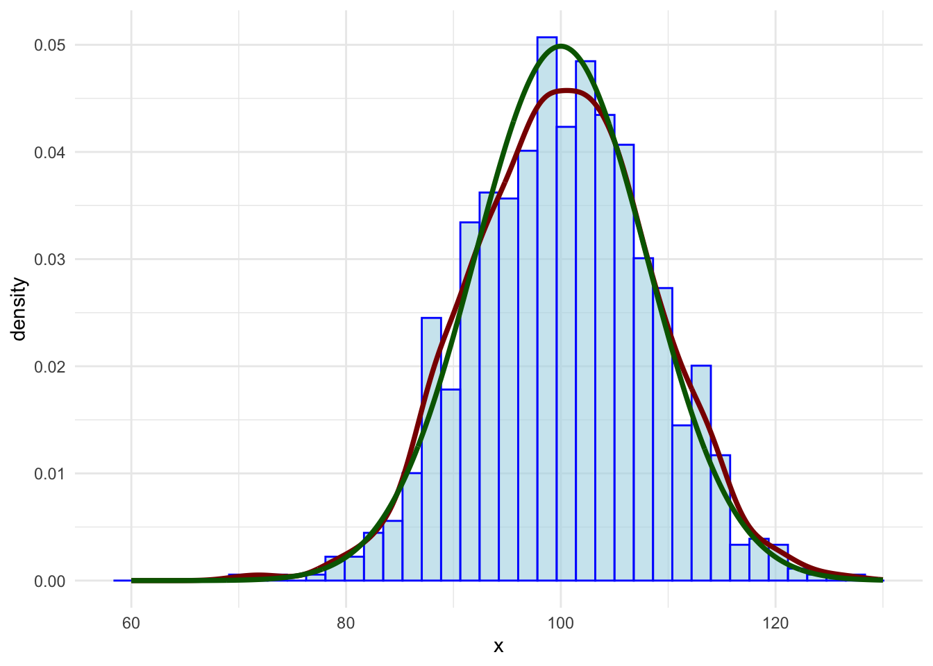

Finally, the pnorm function can be used to find the probability of observing a certain value, or below (or above):

pnorm(q = 100, mean = 100, sd = 8, lower.tail = TRUE)

## [1] 0.5

The value 100 is the mean, so the probability of finding it, or a value below it, is 0.5. One standard deviation should represent 68% of the values:

pnorm(q = 92, mean = 100, sd = 8, lower.tail = TRUE)

## [1] 0.159

(100 - (15.9 * 2) = 68.2)

pnorm(q=120, mean=100, sd=8, lower.tail = FALSE)

## [1] 0.00621

Similarly, there are d, p, q, and r functions for all important distributions:

*binom – binomial
*unif – uniform distribution
*pois – Poisson
*t – Student’s t distribution

Type ?distributions to see a listing of all available ones.

6.2.2 Sampling from vectors or ranges

For random sampling we have the sample and sample.int functions.

The example below samples three values from the numbers between 1 (inclusi) and (inclusive) 5:

sample.int(n=5, size=3)

## [1] 5 2 4

Note that if the number of values you request is larger than the range, you get an error: cannot take a sample larger than the population when 'replace = FALSE'.
You need to use replace = TRUE:

sample.int(n=5, size=10, replace=TRUE)

##  [1] 4 5 3 1 4 3 3 2 4 2

If you provide only a single number, size becomes equal to n, and you get a permutation of the range:

sample.int(5)

## [1] 4 1 3 2 5

The sample() function needs a vector to sample from. For large numbers of values this is of course much less efficient than sample.int(). Here is an example:

sample(x = 1:1000, size = 3)

## [1] 284 461 573

Thus, to sample five rows from a dataframe you would use this technique:

iris[sample.int(n = nrow(iris), size = 5), ]

##     Sepal.Length Sepal.Width Petal.Length Petal.Width    Species
## 109          6.7         2.5          5.8         1.8  virginica
## 145          6.7         3.3          5.7         2.5  virginica
## 39           4.4         3.0          1.3         0.2     setosa
## 63           6.0         2.2          4.0         1.0 versicolor
## 139          6.0         3.0          4.8         1.8  virginica

6.3 General purpose functions

6.3.1 Dealing with NAs

Dealing with NA is a very big thing. When you work with external data there is always the possibility that some values will be missing.

You should be aware that it is not possible to test for NA values (Not Available) values in any other way; using == will simply return NA:

x <- NA
x == NA

## [1] NA

Important functions for dealing with that are na.omit() (drop_na() in dplyr) and complete.cases(). The first drops rows from a dataframe that contain at least one NA; the other returns a logical indicating which rows are complete; i.e. without any NA.
Besides that, many functions in R have a (variant of) the na.rm = argument. For instance, when the sum() function encounters an NA in its input vector, it will always return NA:

x <- c(1, 2, 3, NA)
sum(x)

## [1] NA

sum(x, na.rm = TRUE)

## [1] 6

6.3.2 Convert numeric vector to factor: `cut()`

Sometimes it is useful to work with a factor instead of a numeric vector. For instance, when working with a Body Mass Index (bmi) variable it may be nice to split this into a factor for some analyses. The function cut() is used for this. Suppose you have the following fictitious dataset

## body mass index
bmi <- c(22, 32, 21, 37, 28, 34, 26, 29,
         41, 18, 22, 27, 32, 31, 26)
## year income * 1000 euros
income <- c(23, 14, 20, 13, 47, 15, 38, 29, 
            12, 25, 33, 24, 19, 42, 38)
my_data <- data.frame(bmi = bmi, income = income)

You can of course look at income as a function of bmi using a scatter plot:

with(my_data, plot(income ~ bmi))

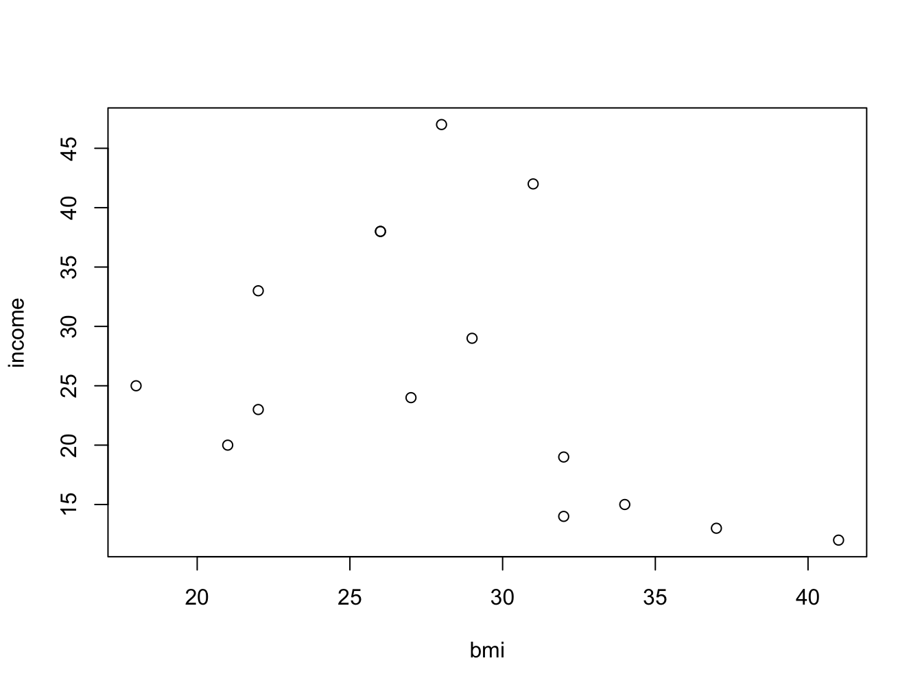
But wouldn’t it be nice to look at the bmi categories as defined by the WHO? To be able to do this, you need to split the numeric bmi variable into a factor using cut().

my_data$bmi_class <- cut(bmi,
    breaks = c(0, 18.5, 25.0, 30.0, Inf), 
    right = F,
    labels = c("underweight", "normal", "overweight", "obese"),
    ordered_result = T)
with(my_data, boxplot(income ~ bmi_class))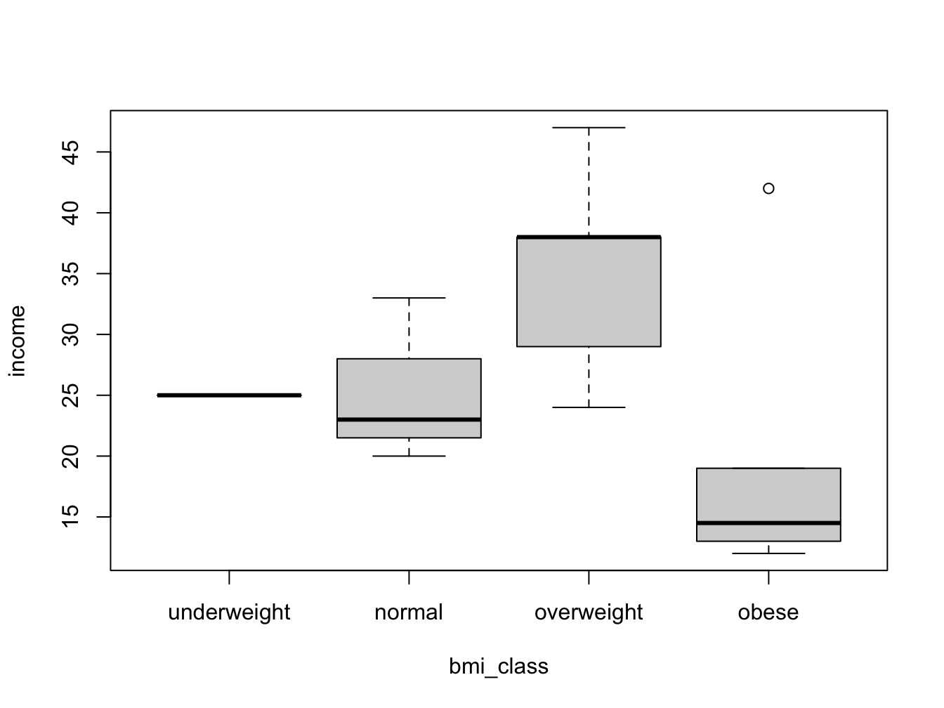

The breaks = argument specifies the split positions; the right = F arguments specifies that the interval is inclusive on the lower (left) boundary:

x <- c(2, 5, 10)
cut(x, breaks = c(0, 2, 5, 10), right = F)

## [1] [2,5)  [5,10) <NA>  
## Levels: [0,2) [2,5) [5,10)

cut(x, breaks = c(0, 2, 5, 10), right = T)

## [1] (0,2]  (2,5]  (5,10]
## Levels: (0,2] (2,5] (5,10]

An interval written as (5,10] means it is from -but excluding- 5 to -but including- 10. Note that in the first example the last value (10) becomes NA because 10 is exclusive in that interval specification.

Memory management

When working with large datasets it may be useful to free some memory once in a while (i.e. intermediate results). Use ls() to see what is in memory; use rm() to delete single or several items: rm(genes), rm(x, y, z) and clear all by typing rm(list = ls())

File system operations

Several functions exist for working with the file system:

getwd() returns the current working directory.
setwd(</path/to/folder>) sets the current working directory.
dir(), dir(path) lists the contents of the current directory, or of path.
A path can be defined as "E:\\emile\\datasets" (Windows) or, on Linux/Mac using relative paths "~/datasets" or absolute paths "/home/emile/datasets".

Glueing character elements: `paste()`

Use paste() to combine elements into a string

paste(1, 2, 3)

## [1] "1 2 3"

paste(1, 2, 3, sep="-")

## [1] "1-2-3"

paste(1:12, month.abb)

##  [1] "1 Jan"  "2 Feb"  "3 Mar"  "4 Apr"  "5 May"  "6 Jun"  "7 Jul"  "8 Aug" 
##  [9] "9 Sep"  "10 Oct" "11 Nov" "12 Dec"

There is a variant, paste0() which uses no separator by default.

A local namespace: `with()`

When you have a piece of related code operating on a single dataset, use with() so you don’t have to type its name all the time.

with(airquality, {
  mdl <- lm(Solar.R ~ Temp)
  plot(Solar.R ~ Temp)
  abline(mdl)
})

Local variables such as mdl will not end up in the global environment.

Writing data to file

To write a data frame, matrix or vector to file, use write.table(myData, file="file.csv"). Standard is a comma-separated file with both column- and row names, unless otherwise specified:

col.names = F
row.names = F
sep = ";"
sep = "\t" # tab-separated

Saving R objects to file

Use the save() function to write R objects to file for later use. This is especially handy with intermediate results in long-running analysis workflows.

x <- stats::runif(20)
y <- list(a = 1, b = TRUE, c = "oops")
save(x, y, file = "xy.RData")

Writing a plot to file

Use one of the functions png(), jpeg(), tiff(), or bmp() for these specific file types. They have widely differing properties, especially with respect to file size.
Use width and height to specify size. Default unit is pixels. Use other unit: units = "mm"

png("/path/to/your/file.png",
    width = 700, height = 350, units = "mm")
plot(cars)
dev.off() # don't forget this one!

A ggplot figure can be written to file like this:

png("myplot.png")
myplot <- ggplot(mtcars, aes(wt, mpg)) + 
  geom_point()
print(myplot)
dev.off()

5 Basics of the ggplot2 package

7 Flow control and scripting